Polar Coordinates
Overview
Polar coordinates can be useful for plotting curves. The origin of this coordinate system is known as the pole. The positive $x$-axis is called the polar axis.
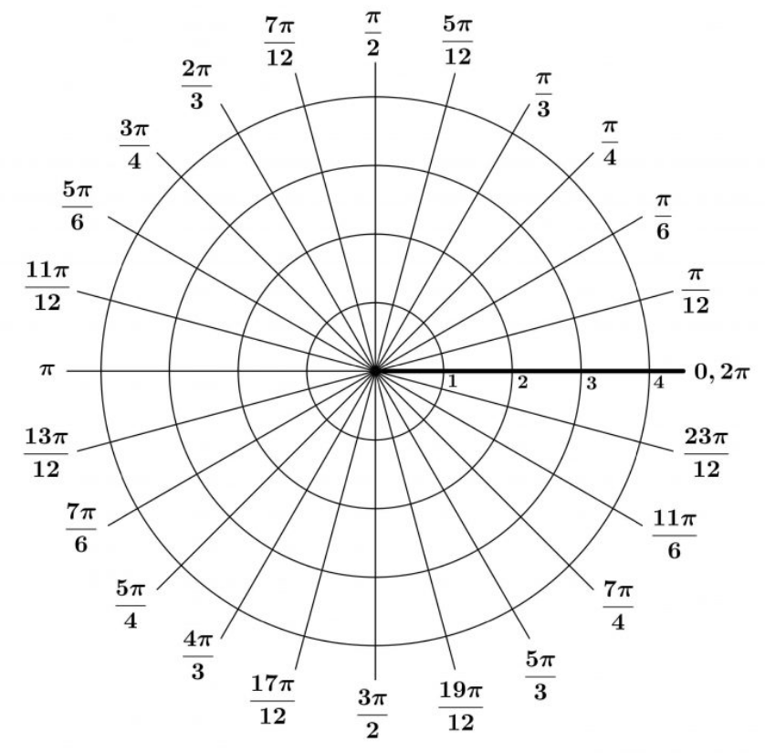
Polar coordinates are of the form $P = (r, \theta)$. The radial coordinate $r$ describes the signed (or directed) distance from the origin to $P$. The angular coordinate $\theta$ describes an angle whose initial side is the positive $x$-axis and whose terminal side lies on the ray passing through the origin and $P$. Positive angles are measured counterclockwise from the positive $x$-axis.
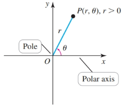
With polar coordinates, points have more than one representation for two reasons. First, angles are determined up to multiples of $2\pi$ radians, so the coordinates $(r, \theta)$ and $(r, \theta \pm 2\pi)$ refer to the same point:
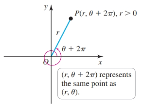
Second, the radial coordinate may be negative. $(r, \theta)$ and $(-r, \theta)$ are reflections of each other through the origin. This means that $(r, \theta), (-r, \theta + \pi)$, and $(-r, \theta - \pi)$ all refer to the same point:

Graphing Polar Coordinates
First, find the angle—counter-clockwise for negative angles and clockwise for positive angles. Next, if the radial coordinate is positive it should be along the terminal side of the angle; otherwise the radial coordinate should be on the reflection of the terminal side i.e. $\theta \pm 2\pi$
We can represent each point in a variety of ways e.g. the point $Q(1, \frac{5\pi}{4})$:
Converting from/to Cartesian coordinates
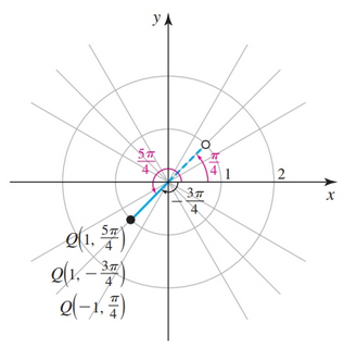
The connection between polar and Cartesian coordinates is shown here:
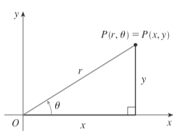
Observe the following:
$$ \cos \theta = \frac{x}{r}\\ \sin \theta = \frac{y}{r} $$And, so we derive the following equations to go from polar to Cartesian coordinates:
$$ x = r \cos \theta\\ y = r \sin \theta $$The $x$ and $y$ equations result in no ambiguities.
We can simply plug in values for $r$ and $\theta$ to obtain the desired coordinate.
We derive the following equations to go from Cartesian to polar coordinates.
$$ x^2 + y^2 = r^2\\ \theta = \tan^{-1} \frac{y}{x} $$This first equation is problematic when we find $\sqrt{r^2} = \pm r$. The second equation is problematic because the range of $\tan^{-1}$ is $(-\pi/2, \pi/2)$. This means the equation will only output values on half of the unit circle i.e. quadrants I and IV.
The strategy for converting from Cartesian to polar is as follows:
- Analyze the ordered pair, and mark the point or determine the appropriate quadrant.
- Find $\theta$.
- Find $\pm r$.
- Choose $r$ or $-r$ such that the polar coordinates correspond to the correct point.
Converting to Cartesian Equations
Strategies
Formulas can be re-expressed by substituting $r^2$ for $x^2 + y^2$:
$$ r^2 = f(\theta) \cdot r\\ x^2 + y^2 = f(\theta) \cdot r $$Some derivations can be expanded with trig identities:
$$ x^2 + y^2 = 6 r \sin \theta\\ x^2 + y^2 = 6y $$Some derivations can be expanded by completing the square:
$$ x^2 + y^2 = 6y\\ x^2 + y^2 - 6y = 0\\ x^2 + y^2 - 6y + 9 - 9 = 0\\ x^2 + (y - 3)^2 = 9\\ $$Graphing Polar Equations
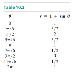
The easiest method is to choose several values of $\theta$, calculate the corresponding $r$-values, and tabulate the coordinates. The points are then plotted and connected with a smooth curve.
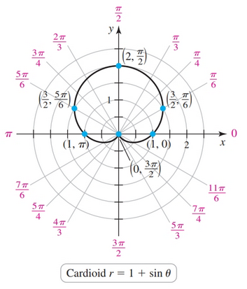
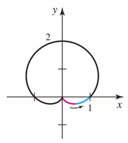
The heart-shaped figure below is known as a cardioid.
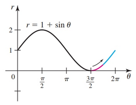
Graphs in Cartesian and Polar coordinates
Cardiod
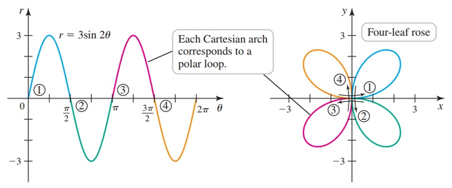
Four-leaf Rose
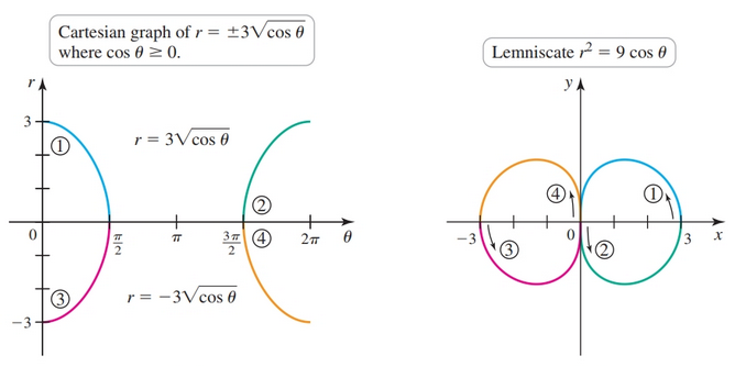
Lemniscate
Polar Equations
Polar equations are often expressed in terms of $\theta$:
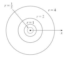
$$ r = f(\theta) $$The graph $r = k$, where $k$ is some constant:
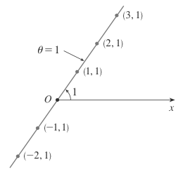
The graph $\theta = k$, where $k$ is some constant:
Converting to Parametric Equations
Given the equations:
$$ x = r \cos \theta\\ y = r \sin \theta $$We can convert from the polar equation $r = f(\theta)$ to parametric equations by substituting in $f(\theta)$:
$$ x = f(\theta) \cos \theta\\ y = f(\theta) \sin \theta $$Tangent Lines
In order to find the derivate (allowing us to find tangent lines) associated with a figure we must first convert to parametric equations. Next, we use the formula for finding the derivative of parametric equations:
$$ \frac{dy}{dx} = \frac{dy/d\theta}{dx/d\theta} $$Recalling that $x = r \cos \theta = f(\theta) \cos \theta$ and $y = r \cos \theta = f(\theta) \cos \theta$ we can come up with a general form:
$$ \frac{dy}{dx} = \frac{d/d\theta[f(\theta) \sin \theta]}{d/d\theta[f(\theta) \cos \theta]} = \frac{f'(\theta) \sin \theta + f(\theta) \cos \theta}{f'(\theta) \cos \theta - f(\theta) sin \theta} $$Note the use of the product rule in both the numerator and denominator.
Recall that when $dy/dx = 0$ the tangent line is horizontal, and when $dy/dx$ is undefined the tangent line is vertical.
Points of Tangency for Vertical and Horizontal Tangent Lines
Given a derivative of $\frac{dy/d\theta}{dx/d\theta}$ we can find the point of tangency of vertical lines of the graph by setting the numerator equal to $0$:
$$ \frac{dx}{d\theta} = 0 $$This gives the angle at which tangency occurs. Next, we plug $\theta$ into $r = f(\theta)$ to obtain the $r$ coordinate.
We use the same strategy to find the point(s) of tangency for horizontal lines, except we use the equation in the numerator:
$$ \frac{dy}{d\theta} = 0 $$Intersection at Origin
If we want to find the angle at which $f(\theta)$ intersects the origin we can set $r = 0$ in $r = f(\theta)$ and solve for $\theta$. Recal that the origin is at $(0, 0)$ and this corresponds to an $r$ of $0$ ($0^2 + 0^2 = 0^2 = 0$).
Strategies
It may be possible to avoid following the general formula for $\frac{dy/d\theta}{dx/d\theta}$ verbatim through trigonometric substitutions. For example, let $f(\theta) = 6 \sin \theta$ so we have:
$$ x = 6 \sin \theta \cos \theta\\ = \overbrace{3 \sin 2 \theta}^{\text{double-angle identity}} y = 6 \sin \theta \theta\\ = 6 \sin^2 \theta $$Our derivative becomes:
$$ \frac{dy}{dx} = \frac{12\sin\theta \cos \theta}{6 \cos 2\theta} $$Area of regions Bounded by Polar Curves
We use the slice-and-sum strategy. Our objective is to find the area of the region $R$ bounded by the graph of $r = f(\theta)$ between the two rays $\theta = \alpha$ and $\theta = \beta$. We assume tat $f$ is continuous and nonnegative on $[\alpha, \beta]$.
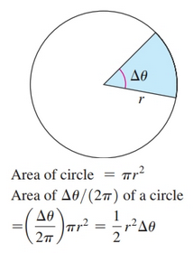
Recall the equation for the sector of a circle.
Approximation
We slice $R$ in the radial direction, creating wedge-shaped slices. The interval $[\alpha, \beta]$ is partitioned into $n$ subintervals by choosing the grid points
$$ \alpha = \theta_0 < \theta_1 < \theta_2 < \dots < \theta_k < \dots \theta_n = \beta $$We let $\Delta \theta_k = \theta_k - \theta_{k - 1}$, for $k = 1, 2, \dots, n$, and we let $\theta_k^*$ be any point of the interval $[\theta_{k - 1}, \theta_k]$. The $k$th slice is approximated by the sector of a circle swept out by an angle $\Delta \theta_k^*
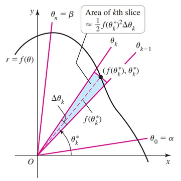
Therefore, the area of the $k$th slice is approximately $\frac{1}{2} f(\theta_k^*)^2 \Delta \theta_k$, for $k = 1, 2, \dots, n$. To find the approximate area of $R$, we sum the areas of these slices:
$$ \text{area} \approx \sum_{k = 1}^n \frac{1}{2} f(\theta_k^*)^2 \Delta \theta_k $$As $n \to \infty$ and $\Delta \theta_k \to 0$ for all $k$, the exact area is given by:
$$ \lim_{n \to \infty} \sum_{k = 1}^n \frac{1}{2} f(\theta_k^*)^2 \Delta \theta_k $$Which can also be expressed as the indefinite integral:
$$ \int_{\alpha}^{\beta} \frac{1}{2} f(\theta)^2 d \theta $$Region Bounded by Two Curves
Given a region bounded by two curves we can use the following formula:
$$ \int_{\alpha}^{\beta} \frac{1}{2} [f(\theta)^2 - g(\theta)^2] d \theta $$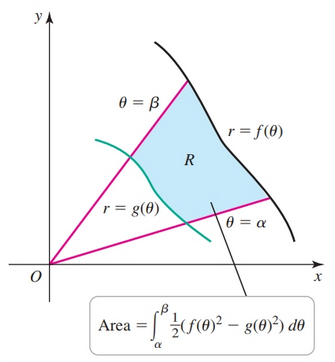
Areas of Polar Regions
Given the functions $g(\theta) = 9 \cos \theta$ and $f(\theta) = 3 + 3\cos \theta$ we can find various areas caused by their intersection. We must find points where these graphs intersect. We do this by setting $f(\theta) = g(\theta)$ and solving for $\theta$. Additionally, we must graph the equations to observe any other points of intersection.
Both functions are graphed below.
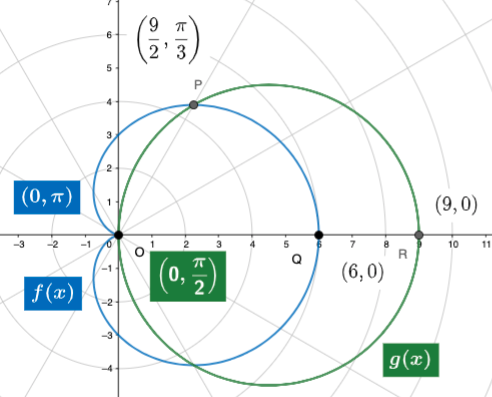
- Note, the point of intersection at $\theta = \frac{\pi}{3}$
- Additionally, the graphs intersect at point $0$ for different values of $\theta$. This demonstrates the need for graphing the two equations as we could not have determined this algebraically.
Area of Combined Regions
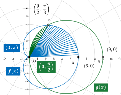
- For $g(x)$ we sweep the area shaded green, from $\frac{\pi}{3}$ to $\pi$.
- For $f(x)$ we sweep the area shaded blue, from $0$ to $\frac{\pi}{3}$.
Area of Right-outside Region
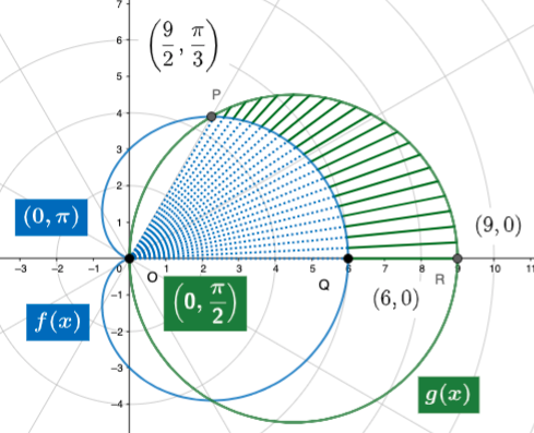
- For $g(x)$ we sweep the area from $0$ to $\frac{\pi}{3}$ (shaded in green).
- We subtract from this the area of $f(x)$ from $0$ to $\frac{\pi}{3}$ (shaded in blue)..
Area of Left-outside Region
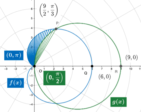
- For the area of $f(x)$ we sweep the from $\frac{\pi}{3}$ to $\pi$ (shaded in blue).
- We subtract the area of $g(x)$ from $\frac{\pi}{3}$ to $\frac{\pi}{2}$ (shaded in green).
Using Symmetry
The equation $r = 2 \cos 2\theta$ is unchanged when $\theta$ is replaced with $-\theta$ (symmetry about the $x$-axis) and when $\theta$ is replaced with $\pi - \theta$ (symmetry about the $y$-axis.
Appealing to symmetry we can find the area of one-half of a leaf and then multiply the result by $8$ to obtain the full rose:

Systems of Equations
Points of Intersection
Given two formulas $f(\theta)$ and $g(\theta)$ the points of intersection must be found by combining two methods:
- Set $f(\theta) = g(\theta)$ and solve for $\theta$.
- Graph the equations.
The second method arises because the graphs may intersect at points for different values of $\theta$.
Sources
- Calculus: Early Transcendentals by Briggs, Cochran, Gillett