Multivariable Calculus
Overview
We have single variable equations, e.g. $f(x) = x^2$.
With multiple variable calculus we deal with equations that handle multiple variables, e.g. $f(x, y) = x^2 + y$.
We are also interested in equations that output vectors, e.g. $f(x, y) = \begin{bmatrix}3x\\2y\end{bmatrix}$.
A convention is that if multiple numbers go into the output (such as the previous equation) think of it as a vector, and in the case of the first equation think of it as a point in a plane. So, think of either point to number or point to vector.
There are several ways to render/visualize that are useful for multivariable calculus.
For example, we have a 2-d input that represents a plane, that gives us the height on the graph:
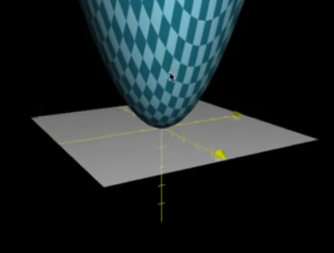
Such a function can also be rendered to a 2-d surface:
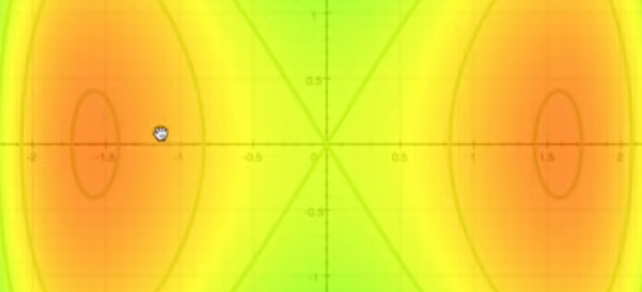
We visualize the entire input space and associate a color with each point. The color tells you roughly the size of the output, and the contour lines tell you which inputs share a constant output value.
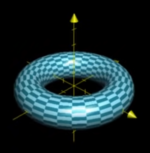
Parametric surfaces allow us to map two dimensional surface such as:

to a three-dimensional one such as:
In a vector field every input point is associated with a vector:
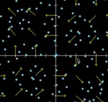
So, we two-dimensional input and two-dimensional output. This can be used to simulate, say, fluid dynamics.
The last example takes inputs in a 2-d space and moves them to an output in two dimensions:

Imagine the plane being folded like paper onto itself.