Limits

Basics of Limits

One description of limits is that they allow us to meaningfully quantify the “tendency” of a function $f(x)$ in instances when we would otherwise use an output, but especially in instances where the function is undefined at the given point.

Consider the function below:

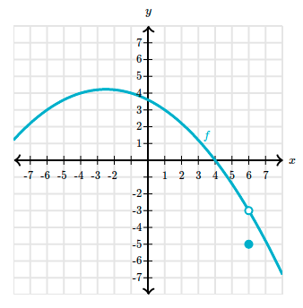
Saying $h(6) = -5$ does not give us insight into the behavior of $h(x)$ near $x = 6$. In fact, we see that the function actually tends toward a different value, $-3$.

We can express the function’s relationship to this missing point by saying that the “limit as $x$ approaches $6$ is $-3$.”

We use a special notation to express this:

$$ \begin{align} \lim_{x \to 6} f(x) = -3 \end{align} $$

Another thing to observe is that we can get infinitely close to $-3$ without ever reaching it.

What do we mean when we say “infinitely close”? We can see how, when the $x$-values are smaller than $3$ but become closer and closer to it, the values of $f$ become closer and closer to $5$

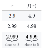
We can also see how, when the $x$-values are larger than $3$ but become closer and closer to it, the values of $f$ become closer and closer to $5$.

Notice that the closest we got to $5$ was with $f(2.999) = 4.999$ and $f(3.001) = 5.001$, which are $0.001$ units away from $5$

We can always get closer to $5$. But that’s exactly what “infinitely close” is all about! Since being “infinitely close” isn’t possible in reality, what we mean by $\lim_{x \to 3} f(x) = 5$ is that no matter how close we want to get to $5$, there’s an $x$-value very close to $3$ that will get us there. We can always get closer and closer to $5$.

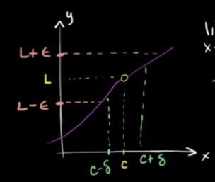
You can get $f(x)$ as “close as you want” to $L$ by making $x$ sufficiently close to $c$.

Note that a function has an infinite number of limits. And, a function has a limit as it approaches a point regardless of whether or not the function is defined at that point.

A variety of situations arise in which limits are helpful for talking about a function.

A limit is commonly expressed as:

$$ \begin{align} \lim_{x \to a} f(x) = L \end{align} $$

We say that “the limit of $f(x)$ as $x$ approaches $a$ is $L$.” Let $f(x)$ be a function defined at all values in an open interval containing $a$, with the possible exception of $a$ itself, and let $L$ be a real number.If all values of the function $f(x)$ approach the real number $L$ as the values of $x \ne a$ approach the number $a$, then we say that the limit of $f(x)$ as $x$ approaches $a$ is $L$. More succinctly, as $x$ gets closer to $a$, $f(x)$ gets closer and stays close to $L$ from both sides of $f(x)$.

The value of $\lim_{x \to a} f(x)$ (if it exists) depends on the values of $f$ near $a$, but it does not depend on the value of $f(a)$. In some cases, the limit $\lim_{x \to a} f(x)$ equals $f(a)$. In other cases, $\lim_{x \to a} f(x)$ and $f(a)$ differ, or $f(a)$ may not even be defined.

When $\lim_{x \to a} f(x) = \lim_{x \to a^+} f(x) = \lim_{x \to a^-} f(x)$ the limit is a two-sided limit i.e. the limit is the same on approach from the right and left. Otherwise, it is not a true limit.

A right-sided limit is a limit that is only approached on the right $\lim_{x \to a^+} f(x) = L$. $x \rightarrow (y)^+$ - ‘as $x$ approaches $y$ from the right’

A left-sided limit is a limit that is only approached on the left $\lim_{x \to a^-} f(x) = L$. $x \rightarrow (y)^-$ - ‘as $x$ approaches $y$ from the left’

Mathematically Rigorous Definition of Limits

In the definition of a limit we want to prove

$$ \begin{align} \lim_{x \to c} f(x) = L \end{align} $$

In the case of a graph where $f(c)$ is undefined, i.e. $\lim_{x \to c} f(x) = L$, consider the case in which need an exacting quantity that gets us sufficiently close to $f(c)$. Now the question we need to answer is: what is the range of acceptable values that we can substitute for $f(c)$–we can get close from two sides. Is a point that is $1$ away enough to substitute for $L$, or do we need something closer such as $.1$

Once we’ve made this decision, e.g. $0.1$, we then need to find an $x$ such that $f(x) = L \pm .01 = L$

The value you that is chosen is $\epsilon$, i.e. you want to get to $L \pm \epsilon$.

Next, we need to find $\delta$, which is the distance to $c$ such that $f(c)$ will be within $\epsilon$ of $L$.

Simply put,

1. Decide how close you want to be to $L$.
2. Find some $\delta$ such that $f(c + \delta) = L \pm \epsilon = L$

Given $\epsilon \gt 0$ we can find $\delta \gt 0$ such that if

$$ \begin{align} |x - c| \lt \delta \to | f(x) - L | \lt \epsilon \end{align} $$

We’ve proved this by showing that no matter $\epsilon$ is chosen, there is a $\delta$.

Continuity

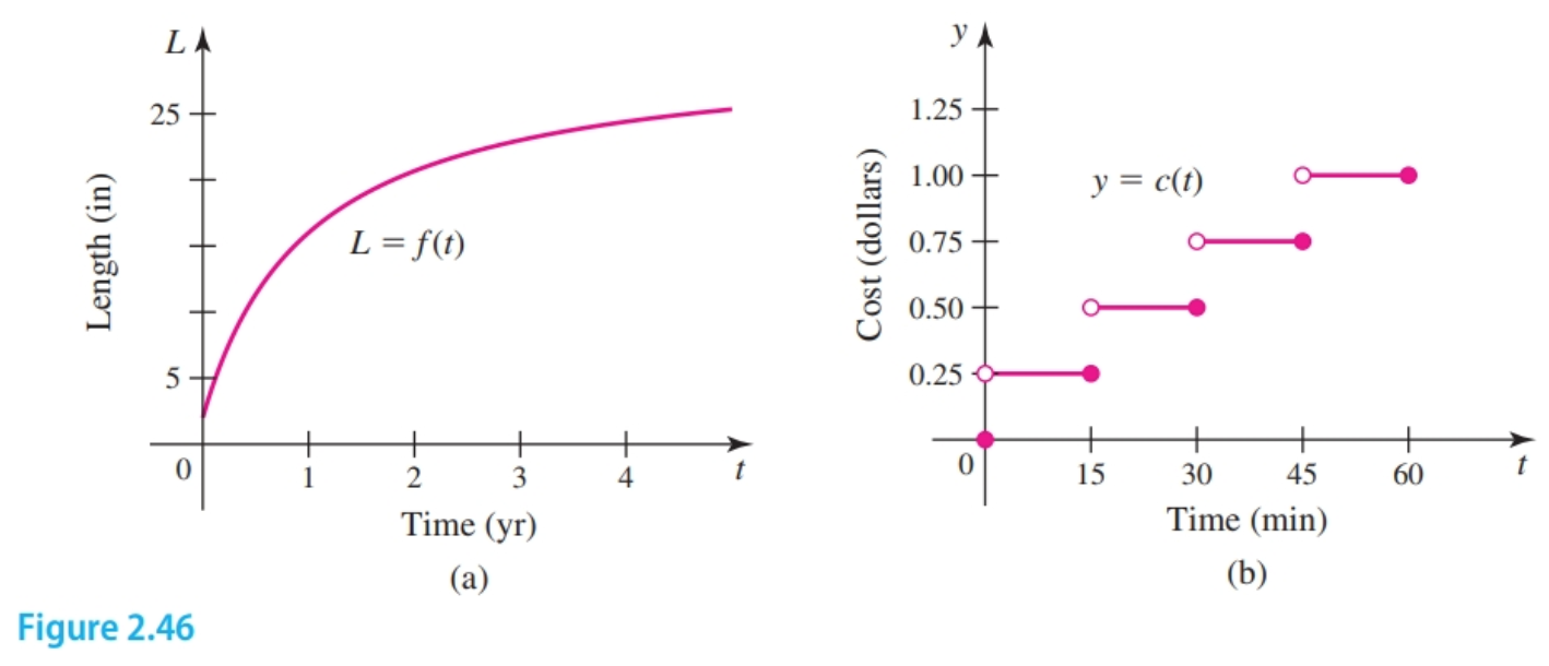
Some graphs are continuous in that they can be drawn as a single line with no holes, jumps, or breaks. Some functions, however, contain abrupt changes in their values.

Continuity at a Point

A function $f$ is continuous at $a$ if $\lim_{x \to a} f(x) = f(a)$. If $f$ is not continuous at $a$, then $a$ is a point of discontinuity.

More specifically, a function is continuous on $a$ if:

1. $f(a)$ is defined ($a$ is in the domain of $f$).
2. $\lim_{x \to a} f(x)$ exists.
3. $\lim_{x \to a} f(x) = f(a)$ (the value of $f$ equals the limit of $f$ at $a$).

The most relevant consequence is that if $f$ is continuous at $a$, then $\lim_{x \to a} f(x) = f(a)$, and direct substitution may be used to evaluate $\lim_{x \to a} f(x)$.

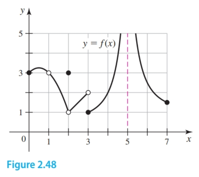
The discontinuities at $x = 1$ and $x = 2$ are called removable discontinuities because they can be removed by redefining the function at these points (in this case, $f(1) = 3$ and $f(2) = 1$). The discontinuity at $x = 3$ is called a jump discontinuity. The discontinuity at $x = 5$ is called an infinite discontinuity.

If $f$ and $g$ are continuous at $a$, then the following functions are also continuous at $a$. Assume $c$ is constant and $n \gt 0$ is an integer.

$f + g$ 2. $f - g$ 3. $cf$ 4. $fg$ 5. $f/g$ provided $g(a) \ne 0$ 6. $(f(x))^n$

A polynomial function is continuous for all $x$. A rational function (a function of the form $\frac{p}{q}$, where $p$ and $q$ are polynomials) is continuous for all $x$ for which $q(x) \ne 0$.

If $g$ is continuous at $a$ and $f$ is continuous at $g(a)$, then the composite function $f \circ g$ is continuous at $a$. Therefore, the limit of $f \circ g$ can be evaluated by direct substitution:

$$ \begin{align} \lim_{x \to a} f(g(x)) = f(g(a)) \end{align} $$

If $g$ is continuous at $a$ and $f$ is continuous at $g(a)$, then

$$ \begin{align} \lim_{x \to a} f(g(x)) = f \left(\lim_{x \to a} g(x) \right) \end{align} $$

If $\lim_{x \to a} g(x) = L$ and $f$ is continuous at $L$, then

$$ \begin{align} \lim_{x \to a} f(g(x)) = f \left(\lim_{x \to a} g(x)\right) \end{align} $$

Continuity on an Interval

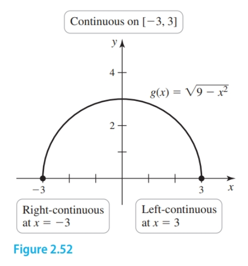
A function $f$ is continuous on an interval $I$ if it is continuous at all points, of $I$. If $I$ contains endpoints, continuity on $I$ means continuous from the right or left at the endpoints–this will be more clear soon.

A function $f$ is continuous from the right (or right-continuous) at $a$ if $\lim_{x \to a^+} f(x) = f(a)$, and $f$ is continuous from the left (or left-continuous) at $b$ if $\lim_{x \to b^-} f(x) = f(b)$.

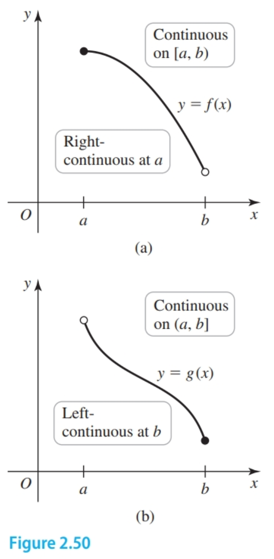
In the figure above $f$ is continuous on the interval $[a, b)$ for the right-continuous function, and continuous on the interval $(a, b]$ for the left-continuous function.

Determining Limits Graphically

Note the following:

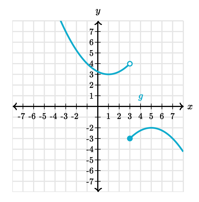
• $\lim_{x \to 3} g(x)$ does not exist.
• There is a left-sided limit: $\lim_{x \to 3^-} g(x) = 4$.
• There is a right-sided limit: $\lim_{x \to 3^+} g(x) = -3$.

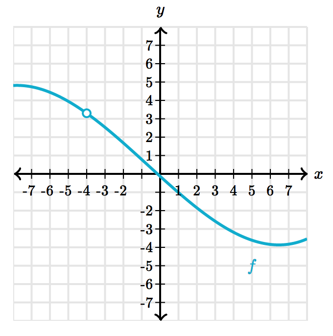
• $\lim_{x \to 4} f(x) = 3.3$

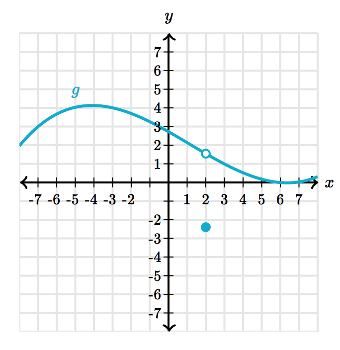
• $\lim_{x \to 2} f(x) = 1.5$

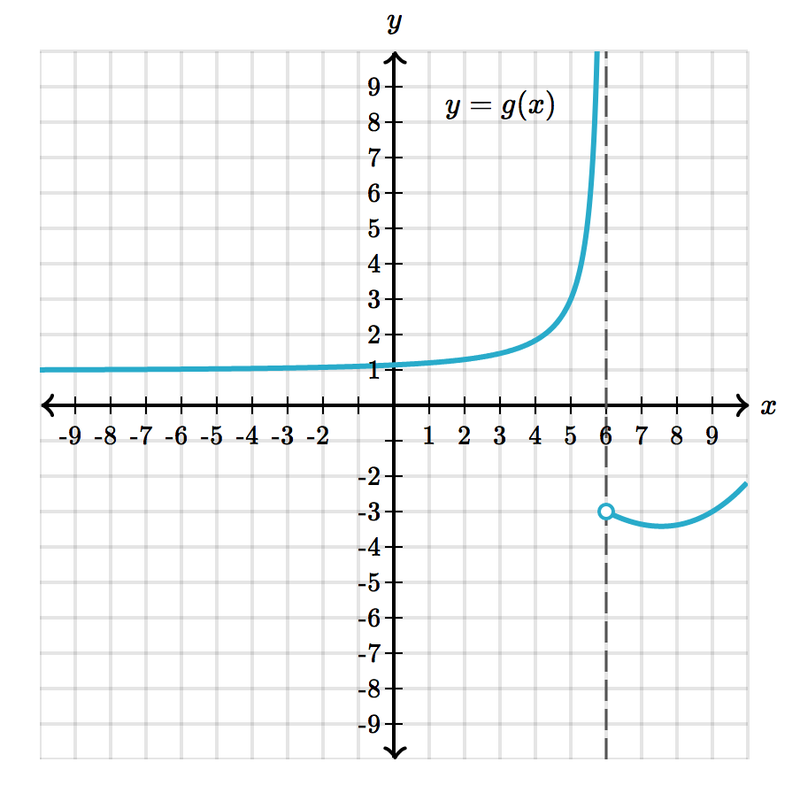
• $\lim_{x \to 6^-} g(x) = \text{unbounded}$

Computing Limits

Limits of Linear Functions

With a linear function we can substitute in values directly to find the limit:

$$ \begin{align} \lim_{x \to a} f(x) = f(a) \end{align} $$

Limit Laws for Combined Functions

Assuming $\lim_{x \to a} f(x)$ and $\lim_{x \to a} g(x)$ exist. The following properties hold, where $c$ is a real number, and $m \gt 0$ and $n \gt 0$ are integers.

1. Sum:

$$ \begin{align} \lim_{x \to a}[f(x) + g(x)] = \lim_{x \to a} f(x) + \lim_{x \to a} g(x) \end{align} $$

2. Difference:

$$ \begin{align} \lim_{x \to a} [f(x) - g(x)] = \lim_{x \to a} f(x) - \lim_{x \to a} g(x) \end{align} $$

3. Constant multiple:

$$ \begin{align} \lim_{x \to a} [cf(x)] = c\lim_{x \to a} f(x) \end{align} $$

4. Product:

$$ \begin{align} \lim_{x \to a} [f(x)g(x)] = \left(\lim_{x \to a} f(x)\right)\left(\lim_{x \to a} g(x)\right) \end{align} $$

5. Quotient:

$$ \begin{align} \lim_{x \to a} \left[\frac{f(x)}{g(x)}\right] = \frac{\lim_{x \to a} f(x)}{\lim_{x \to a} g(x)} \text{ provided } \lim_{x \to a} g(x) \ne 0 \end{align} $$

6. Power:

$$ \begin{align} \lim_{x \to a} [f(x)]^n = \left[\lim_{x \to a} f(x)\right]^n \end{align} $$

7. Fractional power:

$$ \begin{align} \lim_{x \to a} [f(x)]^{\frac{n}{m}} = \left(\lim_{x \to a} f(x)\right)^{\frac{n}{m}} \text{ provided } f(x) \geq 0, \text{ for } x \text{ near } a, \text{ if } m \text{ is even and } n/m \text{ is reduced to lowest terms } \end{align} $$

Law 6 is a special case of Law 7. Letting $m = 1$ in Law 7 gives Law 6.

In Law 7, the limit of $[f(x)]^{\frac{n}{m}}$ involves the $m$th root of $f(x)$ when $x$ is near $a$. If the fraction $n/m$ is in lowest terms and $m$ is even, this root is undefined unless $f(x)$ is nonnegative for all $x$ near $a$, which explains the restrictions shown e.g. there is no solution to $-1^{\frac{n}{m}} = \sqrt[m]{-1^m}$ if $m$ is even.

Polynomial Functions

Also found by direct substitution i.e. $\lim_{x \to a} p(x) = p(a)$

It is now a short step to evaluating limits of rational functions of the form $f(x) = p(x)/q(x)$, where $p$ and $q$ are polynomials. Applying Law 5, we have $\lim_{x \to a} \frac{p(x)}{q(x)} = \frac{\lim_{x \to a} p(x)}{\lim_{x \to a} q(x)} = \frac{p(a)}{q(a)}$, provided $q(a) \ne 0$, which shows that limits of rational functions are also evalutated by direct substitution.

Special Cases

It may be the case that no limit exists and its seems that no meaningful operation can be performed between two functions. However, if the results of evaluating both left and right limits are in agreement we can in fact find the limit:

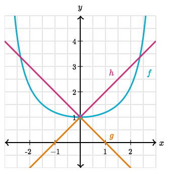
Find $\lim_{x \to -1} (f(x) - h(x))$.

$$ \begin{align} \lim_{x \to -1^-} (f(x) - h(x)) = \lim_{x \to -1^+} (f(x) - h(x)) = 1 \end{align} $$

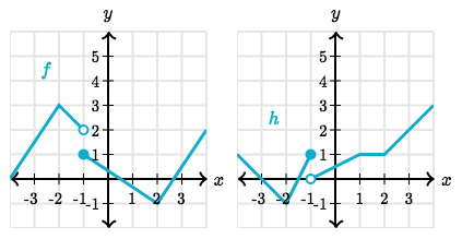
Therefore, $\lim_{x \to -1} (f(x) - h(x)) = 1$.

When direct substitution of a limit $\lim_{x \to a} f(x)$ results in $\frac{k}{0}$ $k \ne 0$, then the limit does not exist and the graph is likely to approach positive or negative $\infty$ as we get closer to $x = a$.

$$ \begin{align} \lim_{x \to -\frac{\pi}{4}} \frac{\cot^2(x)}{1 + \sqrt{2} \sin(x)}\\ = \frac{1}{0} \end{align} $$

When direct substitution of a limit $\lim_{x \to a} f(x)$ results in the indeterminate form $\frac{0}{0}$ then we cannot reason about the limit, and it may or may not exist.

$$ \begin{align} \lim_{x \to -5} \frac{x^2 - 25}{5 + x}\\ = \frac{0}{0} \end{align} $$

Limits of Composite Functions

Given $f(x)$ and $g(x)$ $\lim_{x \to a} (f(g(x))) = \lim_{x \to g(x)} f(x)$ if $\lim_{x \to a} g(x)$ exists and $\lim_{x \to g(x)} f(x)$ exists.

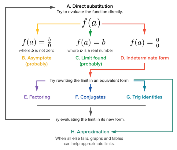
Finding Limits By Substitution

We will need other techniques in finding $\lim_{x \to a} f(x)$ when the limit exists, but $\lim_{x \to a} f(x) \ne f(a)$. One way to evaluate a challenging limit is to replace it with an equivalent limit that can be evaluated by direct substitution.

We update the strategy for finding limits:

Factorization and Cancellation

Some rational functions may not be able to be evaluated with direct substitution. We may be able to factor out a factor in the numerator:

$$ \begin{align} \lim_{x \to 2} \frac{x^2 - 6x + 8}{x^2 - 4} \end{align} $$

Instead, the numerator and denominator are factored; then, assuming $x \ne -2$, we cancel like factors:

$$ \begin{align} f(x) = \frac{x^2 - 6x + 8}{x^2 - 4} \\ = \frac{(x - 2)(x - 4)}{(x - 2)(x + 2)} \\ = \frac{x - 4}{x + 2}, x \ne -2 \end{align} $$

Note that we have substituted the original for a function that doesn’t have a hole at $x = 2$

Rationalization Using Conjugates

The following limit cannot be solved with direct substitution because the denominator is zero at $x = 1$.

$$ \begin{align} \lim_{x \to 1}\frac{\sqrt{x} - 1}{x - 1} \end{align} $$

Instead, we first simplify the function by multiplying the numerator and denominator by the algebraic conjugate of the numerator.

$$ \begin{align} \frac{\sqrt{x} - 1}{x - 1}\\ = \frac{(\sqrt{x} - 1)}{(x - 1)} \cdot \frac{(\sqrt{x} + 1)}{(\sqrt{x} + 1)}\\ \end{align} $$

The new function is not quite the same as the old one:

$$ \begin{align} f(x) = \frac{1}{\sqrt{x} + 1} \end{align} $$

But, we can make it the same:

$$ \begin{align} g(x) = \frac{1}{\sqrt{x} + 1} \text{ for } x \ne 1 \end{align} $$

We can use $f(x)$ to find the limit for the original problem.

Alternate Forms of Trigonmetric Functions

Some problematic trigonometric limits can solved with the help of trigonometric identities.

The following results in the indeterminate form $0/0$:

$$ \begin{align} \lim_{x \to 0} \frac{\sin x}{\sin 2x} \end{align} $$

We can solve by substituting with the trig identity $\sin 2x = 2 \sin x \cos x$ substitution:

$$ \begin{align} \lim_{x \to 0} \frac{\sin x}{2 \sin x \cos x} \end{align} $$

In some instances there is no way to avoid and indeterminate form:

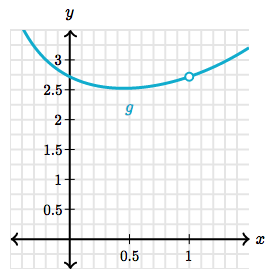
$$ \begin{align} \lim_{x \to 1} \frac{xe^x - e}{x^2 - 1}\\ = \frac{0}{0} \end{align} $$

In this case we can find the approximate limit of $2.75$ with a graph:

Squeeze Theorem

The squeeze theorem or sandwich theorem states that if $g(x) \leq f(x) \leq h(x)$ for all numbers, and at some point $\lim_{x \to c} g(x) = L = \lim_{x \to c} h(k)$, then $f(k)$ must also be equal to $L$. Given a limit such as $\lim_{x \to 0} \frac{x}{\sin(x)}$ where the usual methods fail we can solve it by “squeezing” it in between two other functions such as $g(x) = -|x| + 1$ and $h(x) = |x| + 1$

Infinite Limits

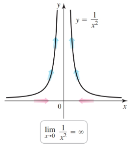
Consider the values of $f(x) = 1/x^2$ in the graph below. As $x$ approaches $0$ from either side, $f(x)$ grows larger and larger. Because $f(x)$ does not approach a finite number as $x$ approaches $0$, $\lim_{x \to 0} f(x)$ does not exist. Nevertheless, we use limit notation and write $\lim_{x \to 0} f(x) = \infty$. The infinity symbol indicates that $f(x)$ grows arbitrarily large as $x$ approaches $0$. This is an example of an infinite limit; in general, the dependent variable becomes arbitrarily large in magnitude as the independent variable approaches a finite number.

If $f(x)$ is negative and grows arbitrarily large in magnitude for all $x$ sufficiently close (but not equal) to $a$, we write

$$ \begin{align} \lim_{x \to a} f(x) = -\infty \end{align} $$

The previous example is a two-sided infinite limit.

There are also one-sided infinite limits e.g. $\lim_{x \to a^+} f(x) = \infty$ (Figure 2.26a).

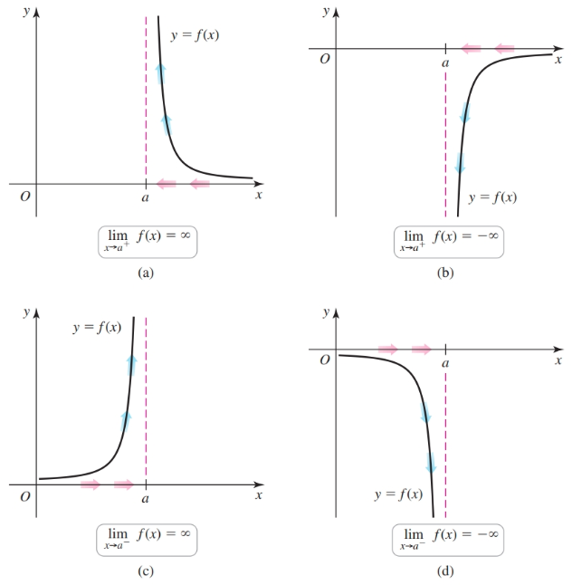
In all the infinite limits illustrated in the figure above, the line $x = a$ is called a vertical asymptote; it is a vertical line that is approached by the graph of $f$ as $x$ approaches $a$.

Many infinite limits are analyzed using a simple arithmetic property: The fraction $a/b$ grows arbitrarily large in magnitude if $b$ approaches $0$ while $a$ remains nonzero and relatively constant. For example, consider the fraction $(5 + x)/x$ for values of $x$ approaching $0$ from the right (Table 2.8).

$$ \begin{array}{ | c | c |} \hline x & \frac{5 + x}{x}\\ 0.01 & \frac{5.01}{0.01} = 501\\ 0.001 & \frac{5.001}{0.001} = 5,001\\ 0.0001 & \frac{5.0001}{0.0001} = 50,001\\ \downarrow & \downarrow \\ 0^+ & \infty \\ \hline \end{array} $$

We see that $\frac{5 + x}{x} \to \infty$ as $x \to 0^+$ because the numerator $5 + x$ approaches $5$ while the denominator is positive and approaches $0$. Therefore, we write $\lim_{x \to 0^+} \frac{5 + x}{x} = \infty$. Similarly, $\lim_{x \to 0^-} \frac{5 + x}{x} = -\infty$ because the numerator approaches $5$ while the denominator approaches $0$ through negative values.

If our function is instead $f(x)= \frac{5 + x}{-x}$, after a simple change of sign, then the situation is reversed and $\lim_{x \to 0^+} \frac{5 + x}{-x} = -\infty$ and $\lim_{x \to 0^-} \frac{5 + x}{-x} = \infty$.

Basically, if $a/b > 0$ as $x \to n^+$ then $\lim_{x \to n^+} f(x) = \infty$ and $\lim_{x \to n^-} f(x) = -\infty$. And, if $a/b < 0$ as $x \to n^+$ then $\lim_{x \to n^+} f(x) = -\infty$ and $\lim_{x \to n^-} f(x) = \infty$.

an algebraic function can have zero, one, or two different slant asymptotes e.g. $f(x) = \frac{x^4}{\sqrt{x^6 + 1}}$ has two slant asymptotes, $y = x$ and $y = -x$.

[slant asymptotes approach infty, a line computed with polynomial division and the original function approach each other as x approaches $\infty$]

We can determine the limits algebraically by testing different values.

Given

$$ \begin{align} h(x) = \frac{3x}{(x + 2)^2} \end{align} $$

We can see that it is unbounded at $x = -2$, i.e. we have an infinite limit.

Testing arbitrary values, e.g. $x = -4, -3, -1, 0$ shows us that

$$ \begin{align} \lim_{x \to -2} h(x) = - \infty \end{align} $$

Limits at Infinity

With limits at infinity, the opposite occurs: The dependent variable approaches a finite number as the independent variable becomes arbitrarily large in magnitude. Limits at infinity determine what is called the end behavior of a function. An application of these limits is to determine whether a system (such as an ecosystem or a large oscillating structure) reaches a steady state as time increases.

In the table below we see that $f(x) = 1/x^2$ approaches $0$ as $x$ increases. In this case, we write $\lim_{x \to \infty} f(x) = 0$.

$$ \begin{array}{ | c | c |} \hline x & f(x) = 1/x^2\\ 10 & 0.01\\ 100 & 0.0001\\ 1000 & 0.000001\\ \downarrow & \downarrow \\ \infty & 0\\ \hline \end{array} $$

The graph below demonstrates the general form of these functions:

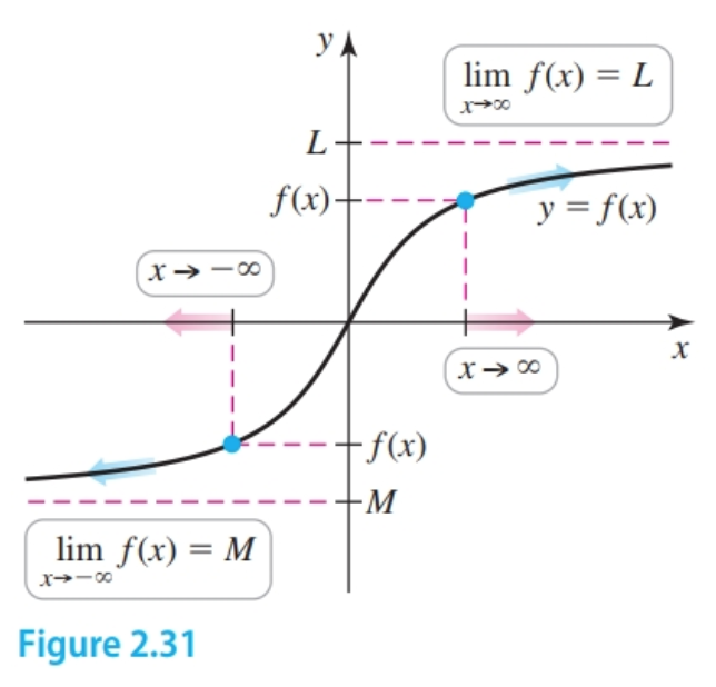
Formally, we can express:

$$ \begin{align} \lim_{x \to \infty} f(x) = L \end{align} $$

We say the limit of $f(x)$ as $x$ approaches infinity is $L$. In this case, the line $y = L$ is a horizontal asymptote of $f$ (Figure 2.31). The limit at negative infinity, $\lim_{x \to -\infty} f(x) = M$, is defined analogously. When this limit exists, $y = M$ is a horizontal asymptote.

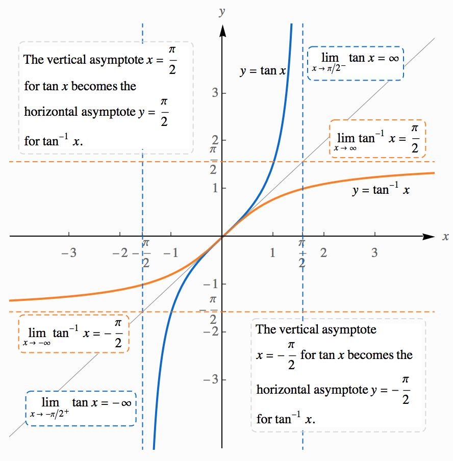
Inverting a graph causes horizontal asymptotes to become vertical asymptotes and vice versa. Note the graph of $y = \tan^{-1}x$ (blue curve) below.

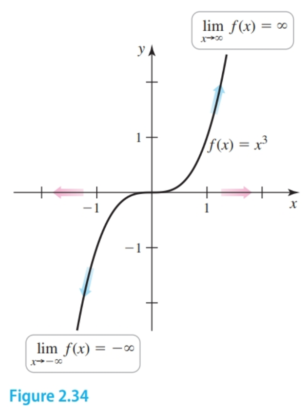
Infinite Limits at Infinity

If $f(x)$ becomes arbitrarily large in magnitude as $x$ becomes arbitrarily large in magnitude then we have an infinite limit at infinity as illustrated by the function $f(x) = x^3$ (Figure 2.34).

Formally, we write

$$ \begin{align} \lim_{x \to \infty} f(x) = \infty \end{align} $$

The limits $\lim_{x \to \infty} f(x) = -\infty$, $\lim_{x \to -\infty} f(x) = \infty$, and $\lim_{x \to -\infty} f(x) = -\infty$ are defined similarly.

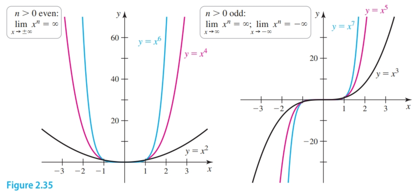
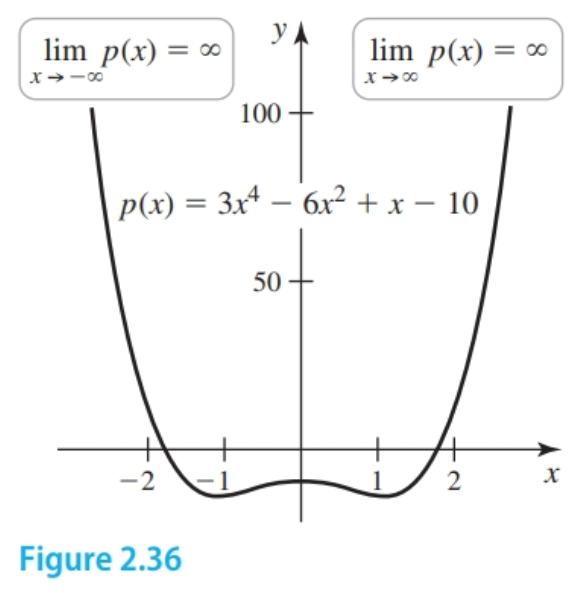
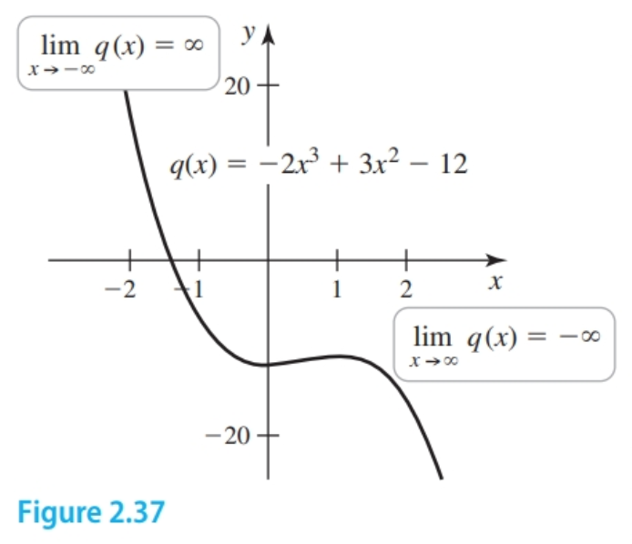
Infinite limits at infinity tell us about the behavior of polynomials for large-magnitude values of $x$. First, consider power functions $f(x) = x^n$, where $n$ is a positive integer. The figure below shows that when $n$ is even, $\lim_{x \to \pm \infty} x^n = \infty$, and when $n$ is odd, $\lim_{x \to \infty} x^n = \infty$ and $\lim_{x \to -\infty} x^n = -\infty$.

It follows that reciprocals of power functions $f(x) = \frac{1}{x^n} = x^{-n}$, where $n$ is a positive integer, behave as follows:

• $\lim_{x \to \infty} \frac{1}{x^n} = \lim_{x \to \infty} x^{-n} = 0$
• $\lim_{x \to -\infty} \frac{1}{x^n} = \lim_{x \to -\infty} x^{-n} = 0$

From here, it is a short step to finding the behavior of any polynomial as $x \to \pm \infty$. Let $p(x) = a_n x^n + a_{n - 1} x^{n - 1} + \dots + a_2 x^2 + a_1 x + a_0$. We now write $p$ in the equivalent form

$$ \begin{align} p(x) = x^n \left(a_n + \frac{a_{n - 1}}{x} + \frac{a_{n - 2}}{x^2} + \dots + \frac{a_0}{x^n} \right) \end{align} $$

More concretely, we can express $p(x) = 5x^4 + 2x^3 + 7x^2 + 3x + 1 = x^4(5 + \frac{2}{x} + \frac{7}{x^2} + \frac{3x}{x^3} + \frac{1}{x^4})$

Notice that as $x$ becomes large in magnitude all the terms except the first term approach zero. Therefore, as $x \to \pm \infty$, we see that $p(x) \approx a_n x^n$ ($5x^4$). This means that as $x \to \pm \infty$, the behavior of $p$ is determined by the term $a_n x^n$ with the highest power of $x$.

We derive the following rules:

1. $\lim_{x \to \pm \infty} x^n = \infty$ when $n$ is even.
2. $\lim_{x \to \infty} x^n = \infty$ and $\lim_{x \to -\infty} x^n$ when $n$ is odd.
3. $\lim_{x \to \pm \infty} \frac{1}{x^n} = \lim_{x \to \pm \infty} x^{-n} = 0$.
4. $\lim_{x \to \pm \infty} p(x) = \lim_{x \to \pm \infty} a_n x^n = \pm \infty$, depending on the degree of the polynomial and the sign of the leading coefficient $a_n$.

End Behavior

The behavior of functions as $x \to \infty$ is an example of what is often called end behavior.

See previous sections for end behavior of polynomials.

Rational Functions

Given a rational function e.g. $\frac{3x + 2}{x^2 - 1}$ we can find the limits at infinity by first dividing both the numerator and denominator by $x^n$, where $x^n$ is the largest term in the denominator.

$$ \begin{align} \frac{\frac{3x}{x^2} + \frac{2}{x^2}} {\frac{x^2}{x^2} - \frac{1}{x^2}} \end{align} $$

From here we determine the following:

$$ \begin{align} = \frac{ \overbrace{ \frac{3}{x} + \frac{2}{x^2}}^{\text{approaches }0}} { 1 - \underbrace{\frac{1}{x^2}}_{\text{approaches }0}} = \frac{0}{1} = 0 \end{align} $$

Therefore, the graph of $f$ has the horizontal asymptote $y = 0$ and $\lim_{x \to -\infty} f(x) = 0$ And, $\lim_{x \to \infty} f(x) = 0$

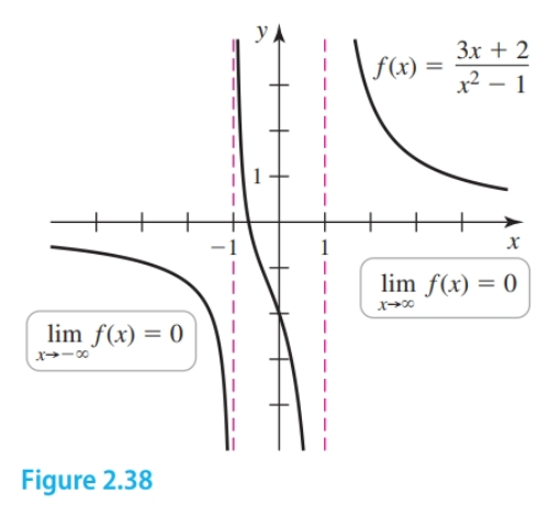
• The limits at infinity and horizontal asymptote for rational functions where the highest-degree in the numerator is greater than the highest degree in the denominator will always be $0$

Given $\frac{40x^4 + 4x^2 - 1}{10x^4 + 8x^2 + 1}$ we can determine the horizontal asymptote to be $4$ and $\lim_{x \to -\infty} f(x) = 4$ And, $\lim_{x \to \infty} f(x) = 4$

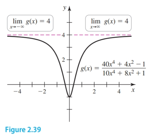
• The limits at infinity and horizontal asymptote for rational functions where the exponent in the highest-degree in the numerator is equal to the exponent in the highest degree in the denominator will always be the coefficient of the highest degree term in the numerator over the coefficient of the highest degree term in the denominator

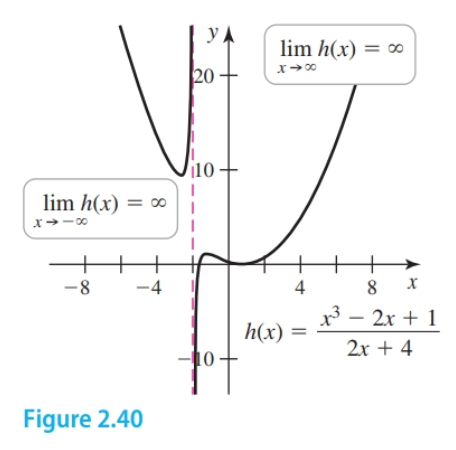
Given $f(x) = \frac{x^3 - 2x + 1}{2x + 4}$ we solve

$$ \begin{align} \frac{\frac{x^3}{x} - \frac{2x}{x} + \frac{1}{x}} {\frac{2x}{x} + \frac{4}{x}}\\ = \frac{\overbrace{x^2}^\text{arbitrarily large} - \overbrace{2}^\text{constant} + \overbrace{\frac{1}{x}}^{\text{approaches }0}} {\overbrace{2}^\text{constant} + \overbrace{\frac{4}{x}}^{\text{approaches } 0}} \end{align} $$

As $x \to \infty$, all the terms in this function either approach zero or are constant—except the $x^2$-term in the numerator, which becomes arbitrarily large. Therefore, the limit of the function does not exist. Using a similar analysis, we find that $\lim_{x \to -\infty} \frac{x^3 - 2x + 1}{2x + 4} = \infty$; These limits are not finite, so the graph of the function has no horizontal asymptote.

• No limit at infinity or horizontal asymptote exists for rational functions where the exponent of the highest-degree in the numerator is greater than the exponent of the highest-degree term in the denominator by $2$ or more.

A special case arises when the exponent of the highest-degree in the numerator is one higher than the highest-degree in the denominator.

Given $f(x) = \frac{2x^2 + 6x - 2}{x + 1}$ we use polynomial long division to divide $2x^2 + 6x - 2$ by $x + 1$ to get the result $2x + 4 - \frac{6}{x + 1}$

As $x \to \infty$, the term $6/(x + 1)$ approaches $0$, and we see that the function behaves like the linear function $l(x) = 2x + 4$. For this reason, the graphs of $f$ and $l$ approach each other as $x \to \infty$a and similarly as $x \to -\infty$. The line described by $l$ is a slant asymptote or oblique asymptote.

In the case of rational functions it is implied that there can be at most one horizontal asymptote.

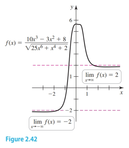
Given the algebraic function $f(x) = \frac{10x^3 - 3x^2 + 8}{\sqrt{25x^6 + x^4 + 2}}$ we use the same strategy and determine the following:

$$ \begin{align} \lim_{x \to \infty} \frac{10x^3 - 3x^2 + 8}{\sqrt{25x^6 + x^4 + 2}}\\ = \frac{ \frac{10x^3}{x^3} - \frac{3x^2}{x^3} + \frac{8}{x^3}} {\sqrt{\frac{25x^6}{x^6} + \frac{x^4}{x^6} + \frac{2}{x^6}}}\\ = \frac{ 10 - \overbrace{\frac{3}{x}}^{\text{approaches } 0} + \overbrace{\frac{8}{x^3}}^{\text{ approaches } 0}} {\sqrt{25 + \overbrace{\frac{1}{x^2}}^{\text{approaches } 0} + \overbrace{\frac{2}{x^6}}^{\text{approaches } 0}}}\\ = \frac{10}{\sqrt{25}} = 2 \end{align} $$

Since as $x \to -\infty$, $x^3$ is negative we divide the numerator and denominator by $-x^3$ to get $-2$.

The limits reveal two asymptotes at $y = 2$ and $y = -2$. Observe that the graph crosses both horizontal asymptotes (Figure 2.42).

If the graph of a function $f$ approaches a line (with finite and nonzero slope) as $x \to \pm \infty$, then that line is a slant asymptote, or oblique asymptote, of $f$.

Given $f(x) = \frac{2x^2 + 6x - 2}{x + 1}$

We first divide the numerator and denominator by the largest power of $x$ appearing in the denominator, which is $x$:

$$ \begin{align} \lim_{x \to \infty} \frac{\frac{2x^2}{x} + \frac{6x}{x} - \frac{2}{x}}{\frac{x}{x} + \frac{1}{x}}\\ = \frac{\overbrace{{2x}^{\text{arbitrarily large}}} + \overbrace{6}^{\text{constant}} - \overbrace{\frac{2}{x}}^{\text{approaches 0}}} {\underbrace{1}_{\text{constant}} + \underbrace{\frac{1}{x}}_{\text{approaches 0}}}\\ = \infty \end{align} $$

A similar analysis shows that $\lim_{x \to \infty} \frac{2x^2 + 6x - 2}{x + 1} = -\infty$. Because these limits are not finite, $f$ has no horizontal asymptote.

If we use polynomial long division the function is written:

$$ \begin{align} f(x) = \underbrace{2x + 4}_{f(x)} - \frac{6}{\underbrace{x + 1}_{\text{approaches 0 as } x \to \infty}} \end{align} $$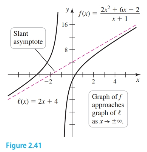

As $x \to \infty$, the term $6/(x + 1)$ approaches $0$, and we see that the function $f$ behaves like the linear function $l(x) = 2x + 4$. For this reason, the graphs of $f$ and $l$ approach each other as $x \to \infty$ (Figure 2.41). A similar argument shows that the graphs of $f$ and $l$ also approach each other as $x \to -\infty$. The line described by $l$ is a slant asymptote; it occurs with rational functions only when the degree of the polynomial in the numerator exceeds the degree of the polynomial in the denominator by exactly $1$.

We can generalize the end behavior and asymptotes of rational functions with the following rules:

a. Degree of numerator less than degree of denominator then $\lim_{x \to \pm \infty} f(x) = 0$ and $y = 0$ is horizontal asymptote. b. Degree of numerator equals degree of denominator then $\lim_{x \to \infty} f(x) = \frac{a}{b}$ where $a$ and $b$ are leading terms of numerator and denominator, respectively. c. Degree of numerator greater than degree of denominator then $\lim_{x \to \pm \infty} f(x) = \infty$ or $-\infty$ and $f$ has no horizontal asymptote. d. Degree of leading term in numerator is $1$ greater than the degree of denominator then $\lim_{x \to \pm \infty} = \infty$ or $-\infty$, with no horizontal asymptote, slant asymptote expressed using polynomial long division. e. Vertical asymptotes when $f$ is in reduced form asymptotes occur at zeros of $q$ in $\frac{p(q)}{q(x)}$

Exponential and Logarithmic Functions

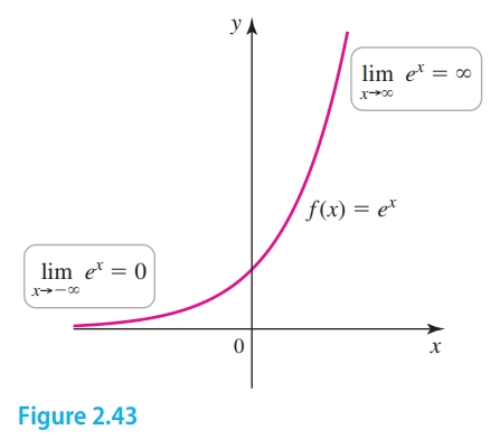
Given the graph $f(x) = e^x$ as $x \to \infty$, $e^x$ increases without bound. All exponential functions $b^x$ with $b > 1$ behave this way. As $x \to -\infty$, the graph of $e^x$ approaches the horizontal asymptote $y = 0$. $e^{-x} = \frac{1}{e^x}$ and so as $x$ approaches $\infty$ $e^{-x}$ approaches the horizontal asymptote $y = 0$. And, as $x$ approaches $-\infty$, $e^{-x}$ approaches $\infty$

The graph of $h(x) = \ln(x)$ is the inverse of $e^x$ and so it is reflected across $y = x$. As $x$ approaches $\infty$, $h(x)$ approaches $\infty$. The domain is $\{x: x > 0\}$. As $x$ approaches $0$, $h(x)$ approaches $-\infty$.

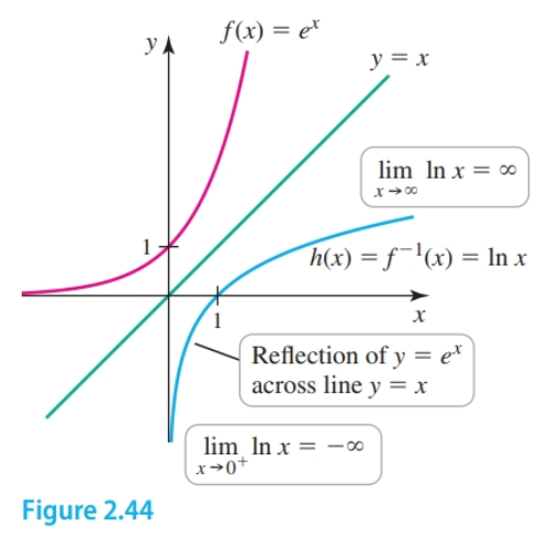
The end behavior of exponential and logarithmic functions can be summarized with the following rules:

1. $\lim_{x \to \infty} e^x = \infty$
2. $\lim_{x \to -\infty} e^x = 0$
3. $\lim_{x \to \infty} e^{-x} = 0$
4. $\lim_{x \to -\infty} e^{-x} = \infty$
5. $\lim_{x \to 0^+} \ln x = -\infty$
6. $\lim_{x \to -\infty} \ln x = \infty$

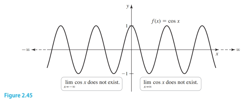
Trigonometric Functions

The graph of $f(x) = \cos x$ oscillates between $-1$ and $1$ as $x \to \infty$ and when $x \to \infty$. Therefore, $\lim_{x \to \infty} \cos x$ does not exist and the same for $\lim_{x \to -\infty} \cos x$.

Now, consider

$$ \begin{gather} \lim_{x \to \infty} \frac{x - 3}{\text{cos}(x) + x} \end{gather} $$

Since $\text{cos}(x)$ oscillates between $-1$ and $1$, we have the following inequality:

$$ \begin{gather} \frac{x - 3}{-1 + x} \le \frac{x - 3}{\text{cos}(x) + x} \le \frac{x - 3}{1 + x} \end{gather} $$

The result is a graph that’s always between the graphs of

$$ \begin{gather} y = \frac{x - 3}{\pm1 + x} \end{gather} $$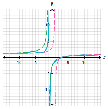

• original function in bold

Since $\lim_{x \to \infty} \frac{x-3}{\pm 1 + x} = 1$, so must our limit be equal to $1$.

So in conclusion,

$$ \begin{gather} \lim_{x \to \infty} \frac{x - 3}{\text{cos}(x) + x} = 1 \end{gather} $$

Continuity of Functions

Functions Involving Roots

Recall that:

$$ \begin{align} \lim_{x \to a} (f(x))^{n/m} = \left(\lim_{x \to a} f(x) \right)^{n/m} \end{align} $$

and if $m$ is even and $n/m$ is reduced then this only applies if $f(x) \geq 0$

Therefore, if $m$ is odd and $f$ is continuous at $a$, then $[f(x)]^{n/m}$ is continuous at $a$:

$$ \begin{align} \lim_{x \to a} (f(x))^{n/m} = \left(\lim_{x \to a} f(x) \right)^{n/m} = (f(a))^{n/m} \end{align} $$

And, if $m$ is even and $n/m$ is reduced then the prior only applies if $f(x) \geq 0$.

When $m$ is even, the continuity of $(f(x))^{n/m}$ must be handled more carefully because this function is defined only when $f(x) \geq 0$.

At points where $f(a) = 0$, the behavior of $(f(x))^{n/m}$ varies. Often we find that $(f(x))^{n/m}$ is left-or right-continuous at that point, or it may be continuous from both sides.

Transcendental Functions

Provided $a$ is in the domain of a function we have $\lim_{x \to a} f(x) = f(a)$ for the following transcendental functions (i.e. we can use direct substitution):

• $\sin x$ and $\sin^{-1} x$
• $\cos x$ and $\cos^{-1} x$
• $\tan x$ and $\tan^{-1} x$
• $\csc x$ and $\csc^{-1} x$
• $\sec x$ and $\sec^{-1} x$
• $\cot x$ and $\cot^{-1} x$
• $b^x$ and $e^x$
• $\log_b x$ and $\ln x$

Trigonometric Functions

$\sin x$ and $\cos x$ are continuous on $(-\infty, \infty)$. Given these facts we can determine that $\sec x$, which is $\frac{1}{\cos x}$ is continuous for all $x$ for which $\cos x \ne 0$ for all $x$ except odd multiples of $\frac{\pi}{2}$. Likewise, the tangent, cotangent, and cosecant functions are continuous at all point of their domains.

The following limits are provable:

$$ \begin{align} \lim_{x \to 0} \frac{\sin x}{x} = 1\\ \lim_{x \to 0} \frac{\cos x - 1}{x} = 0\\ \end{align} $$

Exponential Functions

Until Chapter 6 we assume functions of the form $f(x) = b^x$, with $0 \lt b \lt 1$ or $b > 1$ to be continuous without proof.

Inverse Functions

If a function $f$ is continuous on an interval $I$ and has an inverse on $I$, then its inverse $f^{-1}$ is also continuous (on the interval consisting of the points $f(x)$, where $x$ is in $I$).

Because all the trigonometric functions are continuous on their domains, they are also continuous when their domains are restricted for the purpose of defining inverse functions.

Logarithmic functions of the form $f(x) = log_b x$ are continuous at all points of their domains for the same reason: They are inverses of exponential functions, which are one-to-one and continuous.

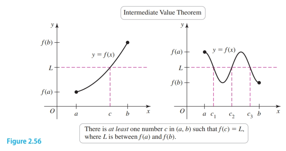
The Intermediate Value Theorem

The existence of solutions to the equation $f(x) = L$ is often established using a result known as the Intermediate Value Theorem. Suppose $f$ is continuous on the interval $[a, b]$ and $L$ is a number strictly between $f(a)$ and $f(b)$. Then there exists at least one number $c$ in $(a, b)$ satisfying $f(c) = L$. Although this theorem is easily illustrated, its proof is beyond the scope of this text.

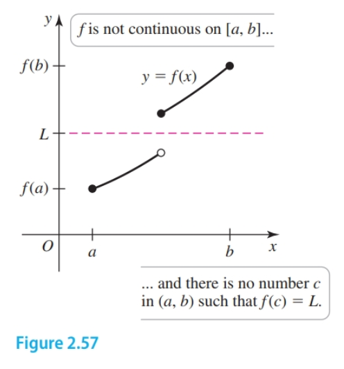
The function $f$ below is not continuous on $[a, b]$. For the value $L$, there is no value of $c$ in $(a, b)$ satisfying $f(c) = L$

Infinite Limits

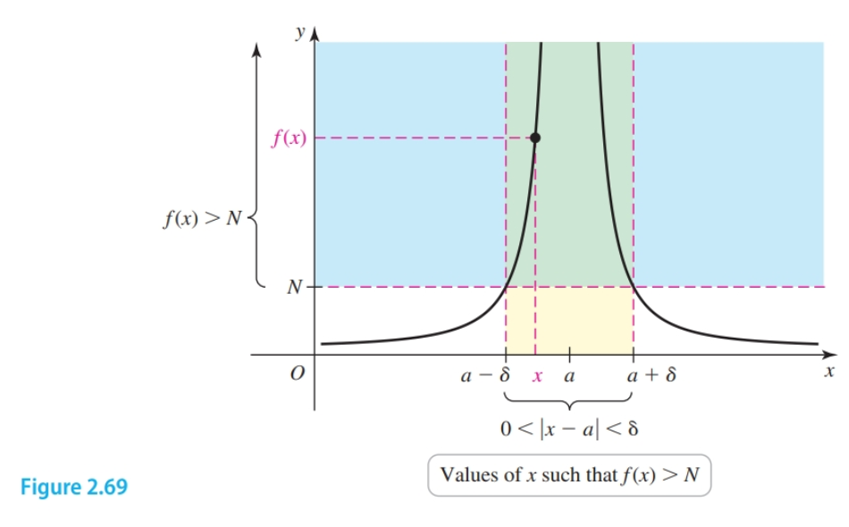
The two-sided infinite limit $\lim_{x \to a} f(x) = \infty$ means that for any positive number $N$, there exists a corresponding $\delta > 0$ such that $f(x) \gt N$ whenever $0 < |x - a| < \delta$

The definitions for the following are similar:

• $\lim_{x \to a} f(x) = -\infty$
• $\lim_{x \to a^+} f(x) = \infty$
• $\lim_{x \to a^+} f(x) = -\infty$
• $\lim_{x \to a^-} = \infty$
• $\lim_{x \to a^-} = -\infty$

For infinite limits, $N$ plays the role that $\epsilon$ plays for regular limits. It sets a tolerance or bound for the function values $f(x)$.

As shown in Figure 2.69, to prove that $\lim_{x \to a} f(x) = \infty$, we let $N$ represent any positive number. Then we find a value of $\delta \gt 0$, depending only on $N$, such that $f(x) \gt N$ whenever $0 \lt |x - a| \lt \delta$.

The process is similar to the two-step process for finite limits.

1. Find $\delta$ Let $N$ be an arbitrary positive number. Use the statement $f(x) > N$ to find an inequality of the form $|x - a| \lt \delta$, where $\delta$ depends only on $N$.
2. Write a proof. For any $N > 0$, assume $0 \lt |x - a| \lt \delta$ and use the relationship between $N$ and $\delta$ found in Step 1 to prove that $f(x) \gt N$.

Given $f(x) \frac{1}{(x - 2)^2}$ we can prove $\lim_{x \to 2} f(x) = \infty$.

Step 1 - Find $\delta$

Assuming $N > 0$, we use the inequality $\frac{1}{(x - 2)^2} > N$ to find $\delta$, where $\delta$ depends only on $N$. Taking the reciprocals of this inequality, it follows that

$$ \begin{align} (x - 2)^2 \lt \frac{1}{N}\\ |x - 2| \lt \frac{1}{\sqrt{n}} \end{align} $$

The inequality $|x - 2| \lt \frac{1}{\sqrt{n}}$ has the form $|x - 2| \lt \delta$ if we let $\delta = \frac{1}{\sqrt{n}}$. We now write a proof.

Step 2 - Write a proof

Given $N > 0$ let $\delta = \frac{1}{\sqrt{N}}$ and assume $0 < |x - 2| \lt \delta = \frac{1}{\sqrt{n}}$. Squaring both sides of the inequality $|x - 2| \lt \frac{1}{\sqrt{n}}$ and taking reciprocals, we have

$$ \begin{align} (x - 2)^2 \lt \frac{1}{N}\\ \frac{1}{(x - 2)^2} \gt N \end{align} $$

We see that for any positive $N$, if $0 \lt |x - 2| \lt \delta = \frac{1}{\sqrt{N}}$, then $f(x) = \frac{1}{(x - 2)^2} \gt N$. It follows that $\lim_{x \to 2} \frac{1}{(x - 2)^2} = \infty$. Note that because $\delta = \frac{1}{\sqrt{N}}$, $\delta$ decreases as $N$ increases.

Limits at Infinity

Precise definitions can also be written for the limits at infinity $\lim_{x \to \infty} f(x) = L$ and $\lim_{x \to -\infty} f(x) = L$.

2.7 Precise Definitions of Limits

Moving Toward a Precise Definition

Recall the definition of a limit is $\lim_{x \to a} f(x) = L$. This means that $f(x)$ is arbitrarily close to $L$ for all $x$ sufficiently close (but not equal) to $a$. In other words $\lim_{x \to a} f(x) = L$ if we can make $|f(x) - L|$ arbitrarily small for any $x$, distinct from $a$, with $|x - a|$ sufficiently small.

We can more formally we express the nature of these conditions with a domain pertaining to $f(x)$ and $L$ and a range pertaining to $x$ and $a$ that are dependent upon one another i.e. we are not talking about $L$ directly, but selecting a criteria that its meets. We use $\epsilon$ to represent the distance between $f(x)$ and $L$, and $\delta$ to represent the distance between $x$ and $a$ and express the limit precisely in the following:

$$ \begin{align} |f(x) - L| < \epsilon \text{ whenever } 0 < |x - a| \lt \delta \end{align} $$

These equations allow us to substitute in a value for $\delta$ or $\epsilon$ and establish a domain of $x$-values that are closer to $a$ in $\lim_{x \to a} f(x) = L$ than $\delta$ and a range of $f(x)$ values that are closer to $L$ than $\epsilon$.

The domain will be $\{ x | a - \delta < x < a + \delta\}$ and the range will be $\{f(x) | L - \epsilon < f(x) < L + \epsilon\}$

We can demonstrate this concept effectively with graphs.

Graphing Limits

We have the limit $\lim_{x \to a} f(x) = L$ such that $|f(x) - 5| < \epsilon$ whenever $0 < |x - 3| \lt \delta$. If we decide to substitute in $1$ for $\epsilon$ our equation for $\epsilon$ becomes $|f(x) - 5| < 1$. We graph the resulting range:

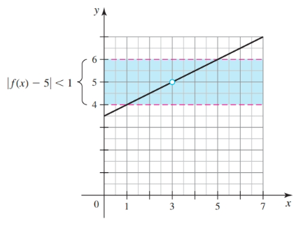
The horizontal lines from our choice of $\epsilon$ delimit a range between $L - 1$ and $L + 1$.

We can easily find a $\delta$ of $2$ that satisfies the definition of the limit by drawing vertical lines that intersect $f(x)$ and the boundaries for the range:

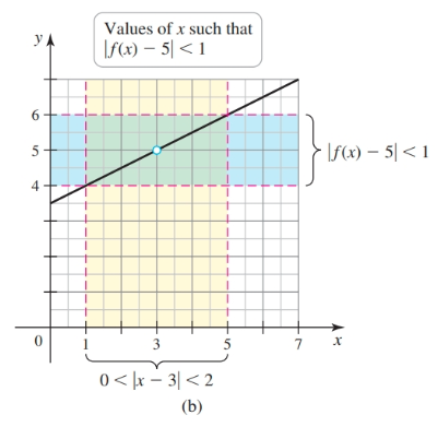
Therefore, $|f(x) - 5 < 1|$ whenever $0 < |x - 3| < 2$

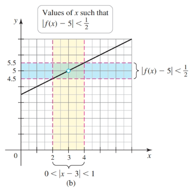
We can decide on a more precise value for $\epsilon$ such as $\frac{1}{2}$ such that the range is described by $|f(x) - 5| < \frac{1}{2}$, and the corresponding $\delta$ is $1$ and the domain described by $0 < |x - 3| < 1$.

Determining Limits Analytically

The new definition defines a limit in terms of a function that allows us to plug in an $\epsilon$ to obtain a $\delta$ such that any value meeting the criterium $0 > |x - a| < \delta$ can be plugged into our new function and $|f(x) - L| < \epsilon$ will be true.

For instance, if we want $|f(x) - L|$ values ($\epsilon$s) $> L - 0.1$ and $< L + 0.1$ we want to to create a function that outputs values $< a + \delta$ and $> a - \delta$. That is we choose $0.1$ for $\epsilon$ and then discover an appropriate $\delta$.

Given the graph of a linear function $f$ with $\lim_{x \to 3} f(x) = 5$ we can determine values of $\delta > 0$ satisfying the statement $|f(x) - 5| \lt \epsilon$ whenever $0 < |x - 3| \lt \delta$ by drawing lines.

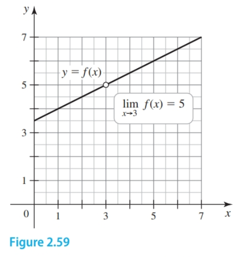
With $\epsilon = 1$, we want $f(x)$ to be less than $1$ unit from $5$, which means $f(x)$ is between $4$ and $6$. We draw the lines $y = 4$ and $y = 6$. To determine a corresponding value of $\delta$ we draw vertical lines that intersect the horizontal lines. These lines happen to be $\pm 2$ units from the limit.

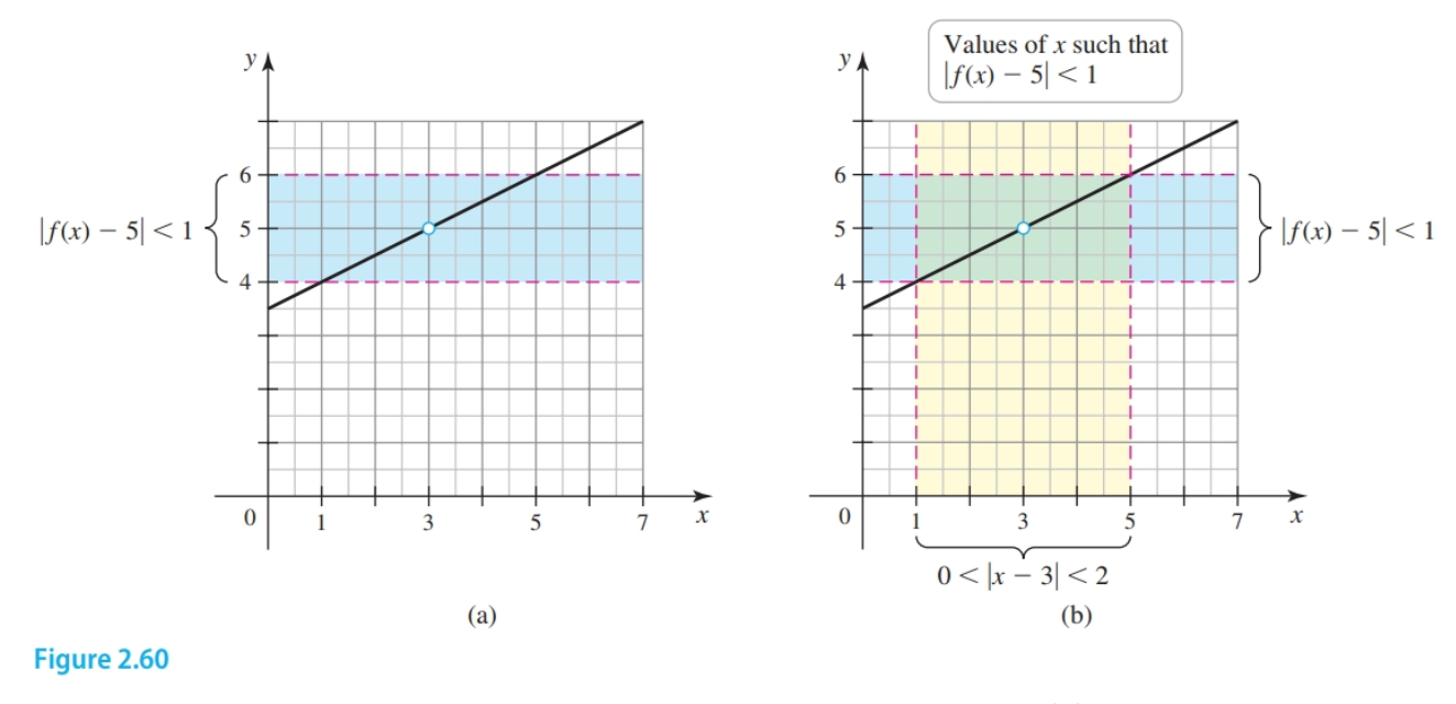
In defining the limit here $\epsilon = 1$, $\delta = 2$.

A Precise Definitio

$\lim_{x \to a} f(x) = L$ means that for any positive number $\epsilon$, there is another positive number $\delta$ such that $|f(x) - L| < \epsilon$ whenever $0 \lt |x - a| \lt \delta$. That is to say that any value plugged into $f(x)$ that meets the second criterium automatically meets the first.

In all limit proofs, the goal is to find a relationship between $\epsilon$ and $\delta$ that gives an admissible value $\delta$, in terms of $\epsilon$ only (i.e. a function). The relationship must work for any positive value of $\epsilon$.

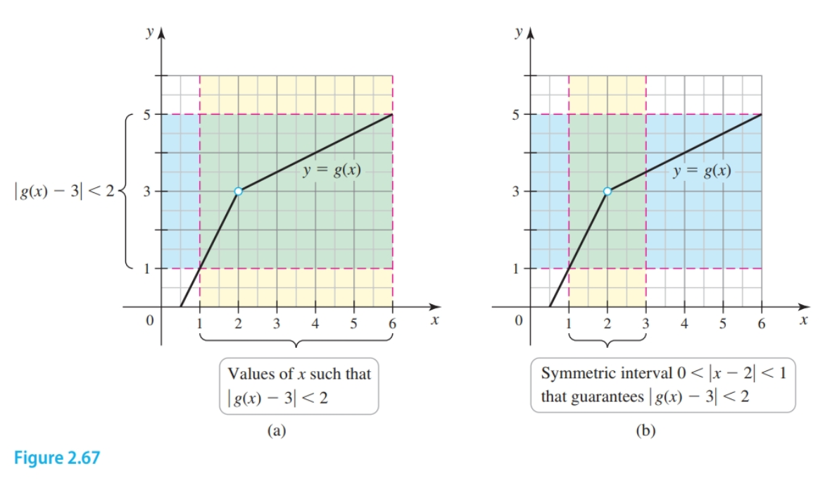
The inequality $0 < |x - a| \lt \delta$ means that $x$ lies between $a - \delta$ and $a + \delta$ with $x \ne a$. We say that the interval $(a - \delta, a + \delta)$ is symmetric about $a$ because $a$ is the midpoint of the interval. Symmetric intervals are convenient, but Example 3 demonstrates that we don’t always get symmetric intervals without a bit of extra work.

Limit Proofs

Steps for proving that $\lim_{x \to a} f(x) = L$

Find $\delta$. Let $\epsilon$ be an arbitrary positive number. Manipulate the inequality $|f(x) - L| < \epsilon$ to find a condition of the form $|x - a| \lt \delta$, where $\delta$ depends only on the value of $\epsilon$. 2. Write a proof. For any $\epsilon > 0$, assume $0 \lt |x - a| < \delta$ and use the relationship between $\epsilon$ and $\delta$ found in Step 1 (i.e. work from the inequality $|x - a|$ to $|f(x) - L|$) to prove that $|f(x) - L| \lt \epsilon$.

We can prove that $\lim_{x \to 4} 4x - 15 = 1$ with the following steps

Step 1 - Scratch Work (Not the Actual Proof)

• Setup inequality with $|f(x) - L|$ and $\epsilon$: $|(4x - 15) - 1| \lt \epsilon$.
• Modify this equation such that the left side resembles $|x - 4|$ ($|x - a|$).

$$ \begin{align} |(4x - 15) - 1| < \epsilon\\ |4x - 16| < \epsilon\\ 4|x - 4| < \epsilon\\ |x - 4| < \frac{\epsilon}{4} \end{align} $$

• Note that we now have $|x - a|$ and we will use this as our $\delta$

Step 2 - Proof

• Given $\epsilon > 0$ choose $\delta = \frac{\epsilon}{4}$. (A series of conditionals follows…)

$$ \begin{align} 0 \lt |x - a| < \delta\\ \to |x - 4| < \frac{\epsilon}{4}\\ \to 4|x - 4| < \epsilon\\ [\text{Steps to arrive at } |f(x) - L|]\\ \to |(4x - 15) - 1| < \epsilon\\ \to |f(x) - L| \lt \epsilon\\ \therefore \lim_{x \to 4} 4x - 15 = 1 \end{align} $$

Justifying Limit Laws

The precise definition of a limit is used to prove the limit laws in Theorem 2.3. Essential in several of these proofs is the triangle inequality states that

$$ \begin{align} |x + y| \leq |x| + |y| \end{align} $$

If $\lim_{x \to a} f(x)$ and $\lim_{x \to a} g(x)$ exist then we can prove that

$$ \begin{align} \lim_{x \to a} (f(x) + g(x)) = \lim_{x \to a} f(x) + \lim_{x \to a} g(x) \end{align} $$

Assume that $\epsilon > 0$ is given. Let $\lim_{x \to a} f(x) = L$, which implies that there exists a $\delta_1 > 0$ such that $|f(x) - L| \lt \frac{\epsilon}{2}$ whenever $0 \lt |x - a| \lt \delta_1$.

Note that because $\lim_{x \to a} f(x)$ exists, if there exists a $\delta > 0$ for any given $\epsilon > 0$, then there also exists a $\delta > 0$ for any given $\frac{\epsilon}{2}$.

Similarly, let $\lim_{x \to a} g(x) = M$, which implies that there exists a $\delta_2 > 0$ such that $|g(x) - M| \lt \frac{\epsilon}{2}$ whenever $0 < |x - a| \lt \delta_2$.

Let $\delta = \min\{\delta_1, \delta_2\}$ and suppose $0 < |x - a| < \delta$. Because $\delta \leq \delta_1$, it follows that $0 \lt |x - a| \lt \delta_1$ and $|f(x) - L| \lt \frac{\epsilon}{2}$. Similarly, because $\delta \leq \delta_2$, it follows that $0 \lt |x - a| \lt \delta_2$ and $|g(x) - M| = \frac{\epsilon}{2}$. Therefore,

$$ \begin{align} |[f(x) + g(x)] - (L + M)| = |f(x) - L) + (g(x) - M)|\\ \leq |f(x) - L| + |g(x) - M|\\ \lt \frac{\epsilon}{2} + \frac{\epsilon}{2} = \epsilon \end{align} $$

We have shown that given any $\epsilon > 04$, if $0 \lt |x - a| \lt \delta$ then $|[f(x) + g(x)] - (L + M)| \lt \epsilon$, which implies that $\lim_{x \to a} [f(x) + g(x)] = L + M = \lim_{x \to a} f(x) + \lim_{x \to a} g(x)$

Sources

• https://www.khanacademy.org/math/differential-calculus
• Calculus: Early Transcendentals by Briggs, Cochran, Gillett