Integral Calculus
Overview
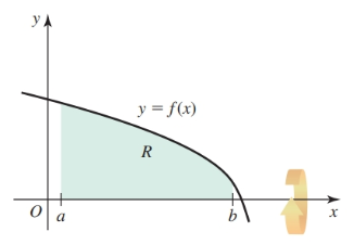
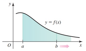
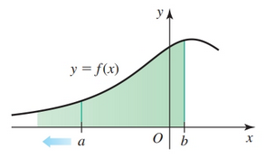
Given the following curve:
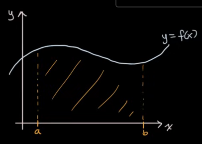
We are interested in finding the area under it from $a$ to $b$.
This is one of the core concerns of integral calculus.
Before we find the answer we need to explore several topics.
Antiderivatives
Going from a derivative $f'$ to a function $f$ is known as antidifferentiation. Given a function $f$, we look for an antiderivative function $F$ whose derivative is $f$; that is, a function $F$ such that $F′ = f$. A function $F$ is an antiderivative of $f$ on an interval $I$ provided $F'(x) = f(x)$, for all $x$ in $I$
$x^2$ is an antiderivative of $2x$ because the derivative of a constant in, say, $x^2 + 5$ is $0$. A function such as $f(x) = 2x$ has an infinite number of antiderivatives including $2x + 1$, $2x + 2$, etc.
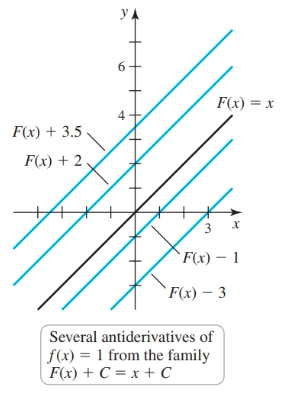
Let $F$ be any antiderivative of $f$ on an interval $I$. Then all the antiderivatives of $f$ on $I$ have the form $F + C$, where $C$ is an arbitrary constant. All antiderivatives of this form comprise a family of antiderivatives.
Indefinite Integral
The indefinite integral is the family of antiderivatives for a given function. The notation that means “find the antiderivatives of $F$” is the indefinite integral:
$$ \begin{align} \int f(x) dx = F(x) + C \end{align} $$“$F(x)$ is the antiderivative or indefinite integral of $f(x)$.”
Every time an indefinite integral sign $\int$ appears, it is followed by a function called the integrand, which in turn is followed by the differential $dx$. For now, $dx$ simply means that $x$ is the independent variable, or the variable of integration. The notation $\int f(x) dx$ represents all the antiderivatives of $f$. The antiderivative AKA indefinite integral of $2x$ is expressed this way:
$$ \begin{align} \int 2x dx = x^2 + C \end{align} $$$C$ is an arbitrary constant called a constant of integration.
Basics of Integration
Given the sum of two antiderivatives, we combine the constants of integration into one constant of integration:
$$ \begin{align} \int f(x) dx + C_1 + \int g(x) dx + C_2\\ \int f(x) dx + \int g(x) dx + C \end{align} $$Linearity properties allow the following operations:
$$ \begin{align} \int [f(x) + g(x)] dx = \int f(x) dx + \int g(x) dx\\ \int k f(x) dx = k \cdot \int f(x) dx, k \in \mathbb{R} \end{align} $$Constants:
$$ \begin{align} \int dx = \int 1 dx = x + C\\ \int k dx = kx + C\\ \end{align} $$Integration of Exponents and Logarithms
The following identities for Indefinite integrals hold (where $a \ne 0$ and $C$ is the constant of integration):
$$ \begin{align} \int x^n dx = \frac{x^{n + 1}}{n + 1} + C, n \ne -1, n \in \mathbb{R}\\ \begin{aligned} \displaystyle\int\sqrt[\Large m]{x^n}\,dx&=\displaystyle\int x^{^{\Large\frac{n}{m}}}\,dx \\\\ &=\dfrac{x^{^{\Large \frac{n}{m}+1}}}{\dfrac{n}{m}+1}+C \end{aligned}\\ \int e^{ax} dx = \frac{1}{a}e^{ax} + C\\ \int x^{-1} dx = \int \frac{1}{x} dx = \int \frac{dx}{x} = \ln |x| + C\\ \int \frac{1}{ax + b} dx = \frac{1}{a} \ln |ax + b| + C\\ \int \ln x dx = x \ln(x) - x + C\\ \int b^x dx = \frac{1}{\ln b} b^x + C, b > 0, b \ne 1\\ \int f(x)f'(x) dx = \frac{1}{n}(f(x))^{n + 1} + C, n \ne -1\\ \end{align} $$Integration of Trig Functions
Indefinite Integrals of Trigonometric Functions (where $a \ne 0, a \in \mathbb{R}$ and $C$ is a constant of integration):
$$ \begin{align} \int \cos x dx = \sin x + C\\ \int \sin x dx = - \cos x + C\\ \int \sec^2 x dx = \tan x + C\\ \int \csc^2 x dx = - \cot x + C\\ \int \sec x \tan x dx = \sec x + C\\ \int \csc x \cot x dx = - \csc x + C\\ \end{align} $$For the above identities any coefficient on $x$ in the left-side term will be found on the right-side on $x$ and in reciprocal form in the front, e.g.:
$$ \begin{align} \int \cos ax dx = \frac{1}{a} \sin ax + C \end{align} $$Some miscellaneous identities:
$$ \begin{align} \int \tan x dx = \ln |\sec x| + C = -\ln |\cos x| + C\\ \int \cot x dx = \ln |\sin x| + C\\ \int \sec x dx = \ln |\sec x + \tan x| + C\\ \int \csc x dx = -\ln |\csc x + \cot x| + C \end{align} $$Integration of Inverse Trigonometric Functions
$$ \begin{align} \int \frac{dx}{\sqrt{a^2 - x^2}} = \sin^{-1} \frac{x}{a} + C\\ \int \frac{dx}{a^2 + x^2} = \frac{1}{a}\tan^{-1} \frac{x}{a} + C\\ \int \frac{dx}{x\sqrt{x^2 - a^2}} = \frac{1}{a} \sec^{-1} \left|\frac{x}{a}\right| + C, a > 0\\ \end{align} $$Strategies for approaching solutions
$$ \begin{align} \int \sqrt{x} dx = \int x^{\frac{1}{2}} dx\\ \int \left(\frac{f(x) + g(x)}{h(x)}\right) dx = \int \left(\frac{f(x)}{h(x)}\right) dx + \int \left(\frac{g(x)}{h(x)}\right) dx\\ \int (x + a)(x + b) dx = \int (x^2 + xa + xb + ab)\\ \end{align} $$Sigma (Summation) Notation
Sigma notation or (summation notation) is used to express sums in a compact way.
The sum $1 + 2 + 3 + \dots + 10$ is represented as $\sum_{k = 1}^{10} k$.
The symbol $\sum$ stands for sum. The index $k$ takes on all the integer values from the lower limit ($k = 1$) to the upper limit ($k = 10$). The expression that immediately follows $\sum$ (the summand) is evaluated for each value of $k$, and the resulting values are summed.
Examples
$$ \begin{align} \sum_{k = 1}^5 k = 1 + 2 + 3 + 4 + 5 = 15\\ \sum_{x = 0}^3 x^2 = 0^2 + 1^2 + 2^2 + 3^2 = 14\\ \sum_{i = 1}^4 (2i + 1) = 3 + 5 + 7 + 9 = 24 \end{align} $$Properties of Sums
The constant multiple rule allows us to factor multiplicative constants out of a sum:
$$ \begin{align} \sum_{k = 1}^n ca_k = c \sum_{k = 1}^n a_k \end{align} $$The addition rule allows us to split a sum into two sums:
$$ \begin{align} \sum_{k = 1}^n (a_k + b_k) = \sum_{k = 1}^n a_k + \sum_{k = 1}^n b_k \end{align} $$Notable Sums
$$ \begin{align} \sum_{k = 1}^n c = cn\\ \sum_{k = 1}^n k = \frac{n(n + 1)}{2}\\ \sum_{k = 1}^n k^2 = \frac{n(n + 1)(2n + 1)}{6}\\ \sum_{k = 1}^n k^3 = \frac{n^2(n + 1)^2}{4}\\ \sum_{i = a}^b c^i = \left\{ \begin{array}{lr} \frac{c^a - c^{b + 1}}{1 - c} & \text{if } c \ne 1\\ b - a + 1 & \text{if } c = 1 \end{array} \right.\\ \sum_{i = 1}^n \frac{1}{i} = \ln n + \gamma, \gamma \approx 0.5772\\ \end{align} $$Example Problems
Expand:
$$ \begin{gather} \displaystyle\sum_{j=0}^3 3-jn=\,? \end{gather} $$We have
$$ \begin{gather} 3 - 0 + 3 - n + 3 - 2n + 3 - 3n \end{gather} $$Consider the sum $2 + 5 + 8 + 11$. What expression is equal to the above sum?
$$ \begin{gather} \displaystyle\sum_{n=1}^4(3n-1) = \displaystyle\sum_{n=0}^3(2+3n) \end{gather} $$Product Summation
With product summation each successive term is multiplied by the previous term.
$$ \begin{align} \prod_{i = 1}^n i = 1 \times 2 \times 3 \times \dots \times n \end{align} $$$$ \begin{gather} \prod_{x=1}^n b^x = b^{\sum_{x=1}^n x} = b^k \end{gather} $$Riemann Sums
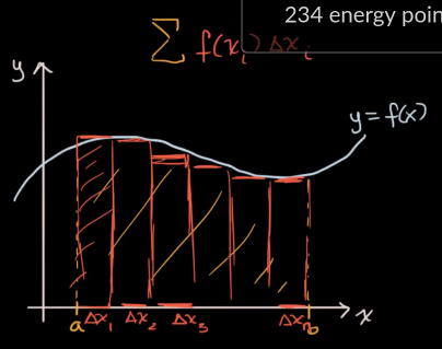
We can approximate “the area under a curve” (aka “the area of the region bounded by the graph of a function”) by dividing the area under the curve into subintervals, forming rectangles from the subintervals, and then summing the areas of the rectangles:
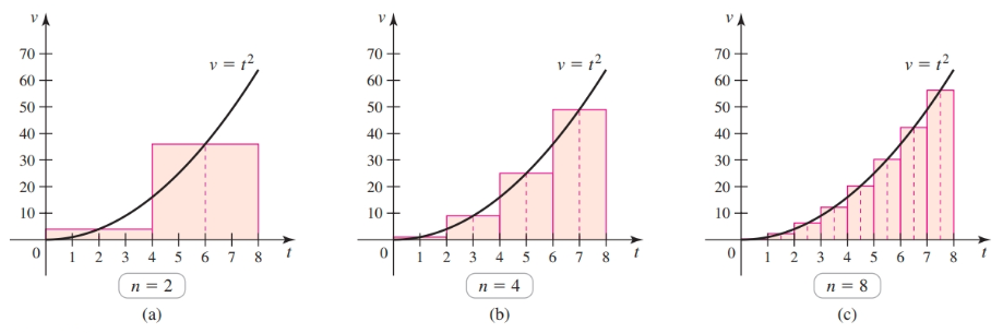
Where $n$ is the number of rectangles, a larger value for $n$ gives a better approximation.
Dividing the interval $[a, b]$ into $n$ subintervals of equal length, we have the intervals:
$$ \begin{align} [x_0, x_1], [x_1, x_2], \dots, [x_{n - 1}, x_n] \end{align} $$Where $a = x_0$ and $b = x_n$. We can express the length of each subinterval $\Delta x$, with the formula:
$$ \begin{align} \Delta x = \frac{b - a}{n} \end{align} $$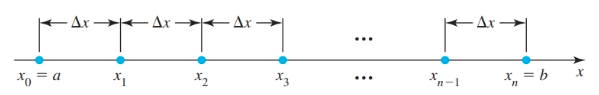
$x_0, x_1, x_2, \dots, x_n$ are known as grid points and they create a regular partition of the interval $[a, b]$. An interval is said to be partitioned into $n$ subintervals.
The $k$th grid point is $x_k = a + k\Delta x$ for $k = 0, 1, 2, \dots, n$
We can find the area of the rectangle in the $k$th subinterval $[x_{k - 1}, x_k]$ with:
$$ \begin{align} \text{height} \cdot \text{base} = f(x_k^{*})\Delta x, \text{ where } k = 1, 2, \dots, n \end{align} $$Summing all of the areas of the subintervals gives us an approximation to the area of $R$, which is called a Riemann sum:
$$ \begin{align} f(x_1^{*}) \Delta x + f(x_2^{*}) \Delta x + \dots + f(x_n^{*}) \Delta x \end{align} $$- The asterisk ($∗$) in the formula is used to indicate that the function $f(x)$ is being evaluated at specific sample points within each subinterval of the partition. The choice of $x_i^∗$, and different choices lead to different types of Riemann sums where the sample point is the left point, right point, midpoint, or any point within the subinterval.
The Riemann sum can be succinctly expressed using sum notation as:
$$ \begin{align} \sum_{k = 1}^n f(x_k^{*})\Delta x \end{align} $$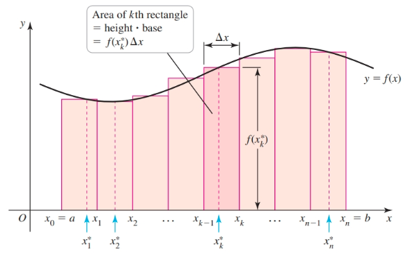
There are three different Riemann sums depending on how the value assigned to $x_k^{*}$ is determined.
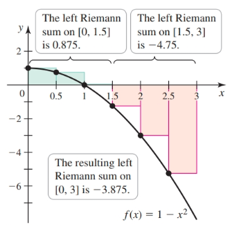
- The sum is called a left Riemann sum if $x_k^{*}$ is the left endpoint of $[x_{k - 1}, x_k]$ i.e. $x_k^* = a + (k - 1)\Delta x$
- The sum is called a right Riemann sum if $x_k^{*}$ is the right endpoint of $[x_{k - 1}, x_k]$ i.e. $x_k^* = a + k \Delta x$
- A sum—which is sometimes more accurate—is called a midpoint Riemann sum if $x_k^{*}$ is the average of $[x_{k - 1}, x_k]$, for $k = 1, 2, \dots, n$ i.e. $x_k^* = a + (k - \frac{1}{2}) \Delta x$—the two endpoints are averaged
Given $f(x) = \sin x$, $\Delta x = \frac{\pi / 2 - 0}{6} = \frac{\pi}{12}$, on the interval $[0, \frac{\pi}{2}]$ and $n = 6$ subintervals:
The left Riemann sum is
$$ \begin{align} (\sin 0) \cdot \frac{\pi}{12} + (\sin \frac{\pi}{12}) \cdot \frac{\pi}{12} + \dots + (\frac{5\pi}{12}) \cdot \frac{\pi}{12}\\ = (\sin 0 + \sin \frac{\pi}{12} + \dots + \sin \frac{5\pi}{12}) \cdot \frac{\pi}{12}\\ \sum_{k = 1}^6 f(0 + (k - 1)\frac{\pi}{12}) \frac{\pi}{12}\\ = 0.863 \end{align} $$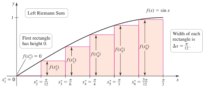
The right Riemann sum is
$$ \begin{align} (\sin \frac{\pi}{12}) \cdot \frac{\pi}{12} + (\sin\frac{\pi}{6}) \cdot \frac{\pi}{12} + \dots + (\sin \frac{\pi}{2}) \cdot \frac{\pi}{12}\\ = (\sin \frac{\pi}{12} + \sin\frac{\pi}{6} + \dots + \sin \frac{\pi}{2}) \cdot \frac{\pi}{12}\\ = \sum_{k = 1}^6 f(0 + k \frac{\pi}{12}) \frac{\pi}{12}\\ = 1.125 \end{align} $$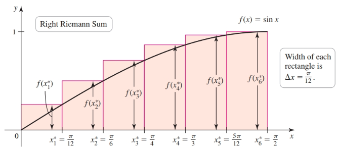
The midpoint Riemann sum is
$$ \begin{align} (\sin \frac{\pi}{24}) \cdot \frac{\pi}{12} + (\sin \frac{3\pi}{24}) \cdot \frac{\pi}{12} + \dots + (\sin \frac{11\pi}{24}) \cdot \frac{\pi}{12}\\ = (\sin \frac{\pi}{24} + \sin \frac{3\pi}{24} + \dots + \sin \frac{11\pi}{24}) \cdot \frac{\pi}{12}\\ \sum_{k = 1}^6 f(0 + (k - \frac{1}{2}) \frac{\pi}{12}) \frac{pi}{12}\\ = 1.003 \end{align} $$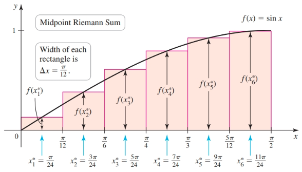
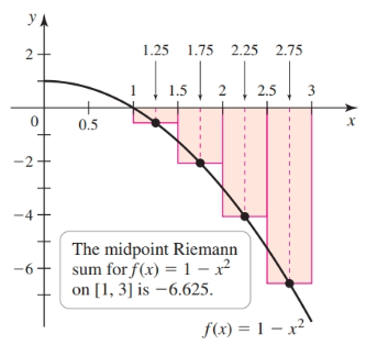
When a function is increasing on interval $[a, b]$, the left Riemann sum underestimates the area under a curve while the right Riemann sum overestimates the area under a curve. The midpoint Riemann sum usually provides the best estimate.
Given an area under a curve whose $y$ values are negative, Riemann sums approximate the negative of the area:
Given an area under a curve with $y$-values that are positive and negative, the Riemann sums of the positive part of the curve work against the negative part to create the net area AKA signed area of the region. This is the difference between the area above the $x$-axis and the area below the $x$-axis. To find net area, we add negative and positive results for the sums together to obtain a value in between.
General Riemann Sum
A general partition of $[a, b]$ consists of the $n$ subintervals:
$$ \begin{align} [x_0, x_1], [x_1, x_2], \dots, [x_{n - 1}, x_n] \end{align} $$where $x_0 = a$ and $x_n = b$.
Further,
$$ \begin{align} a = x_0 < x_1 < x_2 < \dots < x_{n - 1} < x_n = b \end{align} $$The length of the $k$th subinterval is $\Delta x_k = x_k - x_{k - 1}$, for $k = 1, \dots, n$. In contrast to a regular partition we let $x_k^*$ be any point in the subinterval $[x_{k - 1}, x_k]$.
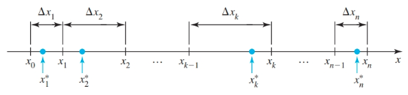
If $f$ is defined on $[a, b]$, the sum
$$ \begin{align} \sum_{k = 1}^n f(x_k^*) \Delta x_k = f(x_1^*) \Delta x_1 + f(x_2^*) \Delta x_2 + \dots + f(x_n^*) \Delta x_n \end{align} $$is called a general Riemann sum for $f$ on $[a, b]$
As was the case for regular Riemann sums, there are left, right, and midpoint Riemann sums.
Introduction to Integrals
We revisit the curve from earlier:
Again, we are interested in finding the area under it from $a$ to $b$.
How do we do this?
We could divide the graph up by hand…
And, this would give us a pretty good approximation. Obviously, we can get a better approximation with smaller $x$s and more $\Delta x$s. What if instead we found the limit of this as $n$ approaches infinity:
$$ \begin{gather} \lim_{n \to \infty} \sum_{i=1}^n f(x_i) \Delta x_i \end{gather} $$This is the core idea of integral calculus. The summation above is known as “the integral from $a$ to $b$ of $f(x) dx$,” and is usually expressed as:
$$ \begin{gather} \int_{a}^b f(x) dx \end{gather} $$You can view the integral sign as like the “s” in the sigma notation. But, instead of taking the sum of a discrete number of things, we’re taking the sum of an infinite number of infinitely thin things. Instead of $f(x)$ times $\Delta x$, you now have $f(x)$ times $dx$, which represents infinitesimally small things.
The concept of the integral is closely tied to that of the derivative. Instead of starting with a function and going to a derivative, we will often be going from a derivative back to the original function – the antiderivative.
The definite integral can be used to express information about accumulation and net change in applied contexts.
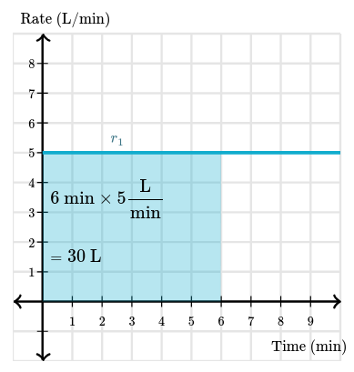
Say a tank is being filled with water at a constant rate of $\blueD{5\text{ L/min}}$ (liters per minute) for $6 \text{min}$. We can find the volume of the water (in $\text{L}$) by multiplying the time and the rate:
$$ \begin{gather} \begin{aligned} \text{Volume}&=\maroonD{\text{Time}}\times\blueD{\text{Rate}} \\ &=\maroonD{6\,\text{min}}\cdot\blueD{5\,\dfrac{\text{L}}{\text{min}}} \\ &=30\dfrac{\cancel{\text{min}}\cdot\text{L}}{\cancel{\text{min}}} \\ &=30\,\text{L} \end{aligned} \end{gather} $$Now consider this case graphically. The rate can be represented by the constant function $r_1(t) = 5$.
The area of the rectangle bounded by the graph of $r_1$ and the horizontal axis between $t = 0$ and $t = 6$ gives us the volume of water after $6$ minutes:
Now say another tank is being filled, but this time the rate isn’t constant:
$$ \begin{gather} r_2(t)=6\sin(0.3t) \end{gather} $$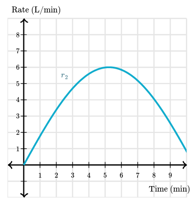
Again, we can approximate this with a Riemann sum:
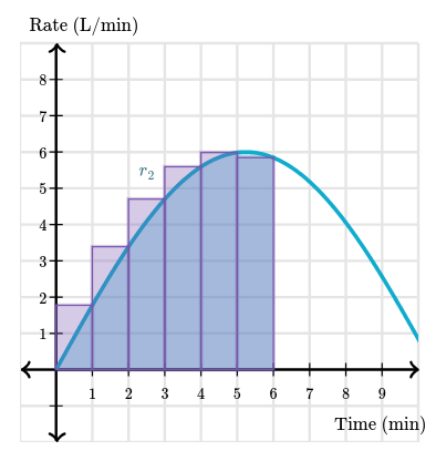
As we use more rectangles with smaller widths, we will get a better approximation. If we take this to a limit of accumulating infinite rectangles, we will get the definite integral $\int_{0}^6 r_2(t) dt$. This means that the exact volume of water after $6$ minutes is equal to the area bounded by the graph of $r_2$ and the horizontal axis between $t = 0$ and $t = 6$.
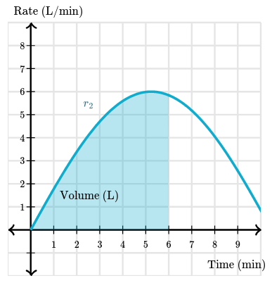
And so, integral calculus allows us to find the total volume after $6$ minutes:
$$ \begin{gather} \begin{aligned} \displaystyle\int_0^6 r_2(t)\,dt&=\displaystyle\int_0^6 6\sin(0.3t)\,dt \\\\ &=-\dfrac{6}{0.3}\Big[\cos(0.3t)\Big]_0^6 \\\\ &=-\dfrac{6}{0.3}\Big[\cos(1.8)-\cos(0)\Big] \\\\ &\approx 24.5\,\text{L} \end{aligned} \end{gather} $$Definite integral of the rate of change of a quantity gives the net change in that quantity.
We had a function that describes a rate. In our case, it was the rate of volume over time. The definite integral of that function gave us the accumulation of volume—that quantity whose rate was given. Another important feature here was the time interval of the definite integral. In our case, the time interval was the beginning ($t =0$) and $6$ minutes after that ($t = 6$). So the definite integral gave us the net change in the amount of water in the tank between $t = 0$ and $t = 6$.
These are the two ways we commonly think about definite integrals: they describe an accumulation of a quantity, so the entire definite integral gives us the net change in that quantity.
Again, the definite integral always gives us the net change in a quantity, not the actual value of that quantity. To find the actual quantity, we need to add an initial condition to the definite integral.
If the tank was empty, then $\int_{0}^6 r_2(t) dt \approx 24.5$ is really the amount of water in the tank after $6$ minutes. But if the tank already contained, say, $7$ liters of water, then the actual volume of water in the tank after $6$ minutes is:
$$ \begin{gather} \underbrace{7}_{\text{volume at }t=0}+\overbrace{\displaystyle\int_0^6 r_2(t)\,dt}^{\text{change in volume from }t=0\text{ to }t=6} \end{gather} $$This is approximately $7+24.5=31.5\text{ L}$.
Definite Integral
The definite integral can be used to express information about accumulation and net change in applied contexts.
It is reasonable to expect the Riemann sum approximations to approach the exact value of the net area as the number of subintervals $n \to \infty$ and as the length of the subintervals $\Delta x \to 0$. In terms of limits we write:
$$ \begin{align} \text{net area } = \lim_{n \to \infty} \sum_{k = 1}^n f(x_k^*) \Delta x \end{align} $$Now, consider the limit of, a general Riemann sum, $\sum_{k = 1}^n f(x_k^*) \Delta x_k$ as $n \to \infty$ and as all the $\Delta x_k \to 0$. We let $\Delta$ denote the largest value of $\Delta x_k$; that is, $\Delta = max \{ \Delta x_1, \Delta x_2, \dots, \Delta x_n\}$. Observe that if $\Delta \to 0$, then $\Delta x_k \to 0$, for $k = 1, 2, \dots, n$. For the limit $\lim_{\Delta \to 0} \sum_{k = 1}^n f(x_k^*)\Delta x_k$ to exist, it must have the same value over all general partitions of $[a, b]$ and for all choices of $x_k^*$ on a partition.
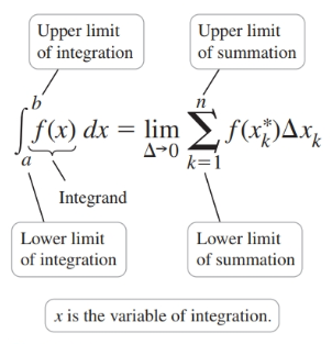
A function $f$ defined on $[a, b]$ is integrable on $[a, b]$ if $\lim_{\Delta \to 0} \sum_{k = 1}^n f(x_k^*) \Delta x_k$ exists and is unique over all partitions of $[a, b]$ and all choices of $x_k^*$ on a partition. This limit is the definite integral of $f$ from $a$ to $b$, which we write as
$$ \begin{align} \int_a^b f(x) dx = \lim_{\Delta \to 0} \sum_{k = 1}^n f(x_k^*) \Delta x_k, [a, b] \end{align} $$There is a direct match on either side of the equation. In the limit as $\Delta \to 0$, the finite sum, denoted $\Sigma$, becomes a sum with an infinite number of terms, denoted $\int$—an elongated $S$ for sum. The limits of integration, $a$ and $b$, and the limits of summation also match: the lower limit in the sum, $k = 1$, corresponds to the left endpoint of the interval, $x = a$, and the upper limit in the sum, $k = n$, corresponds to the right endpoint of the interval, $x = b$. The function under the integral sign is called the integrand. Finally, the differential $dx$ in the integral (which corrsponds to $\Delta x_k$ in the sum) is an essential part of the notation; it tells us that the variable of integration is $x$. It is a dummy variable that is completely internal to the integral. It must only not be in conflict with other variables that are in use.
Theorem: If $f$ is continuous on $[a, b]$ or bounded on $[a, b]$ with a finite number of discontinuities, then $f$ is integrable on $[a, b]$.
We can express limits of sum this way:
$$ \begin{align} \lim_{\Delta \to 0} \sum_{k = 1}^n (3x_k^{*2} + 2x_k^* + 1) \Delta x_k \end{align} $$This is called definite integral and can also be expressed this way:
$$ \begin{align} \int_1^3 (3x^2 + 2x + 1) dx \end{align} $$Properties of Definite Integrals
Let $f$ and $g$ be integrable functions on an interval that contains $a$, $b$, and $p$.
Definite Integral over a Single Point
$$ \begin{gather} \int_a^a f(x) dx = 0\\ \end{gather} $$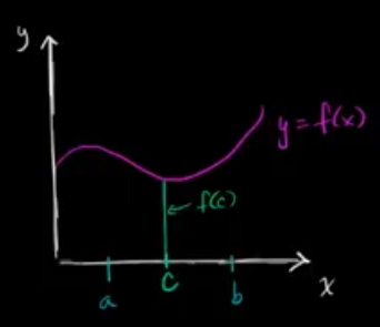
Negative Definite Integrals
$$ \begin{gather} \int_a^b f(x) dx = - \int_b^a f(x) dx\\ \end{gather} $$$$ \begin{gather} \lim_{n \to \infty} \sum_{i=1}^n f(x_i) \Delta x \text{ where } \Delta X = \frac{b - a}{n} \end{gather} $$Now that $\Delta x = \frac{a - b}{n}$, $\Delta x$ will be negative and therefore the integral will be negative.
Given $g(x) = \int_0^x f(t) dt$, $g(-2) = \int_0^{-2} f(t) dt = - \int_{-2}^0 f(t) dt$.
Similarly, given $g(x) = \int_x^3 f(t) dt$, $g'(x) = \frac{d}{dx} \left[- \int_3^x f(t) dt \right]$.
Scaled version of function
$$ \begin{gather} \int_a^b c f(x) dx = c \int_a^b f(x) dx, \text{ any constant }C \end{gather} $$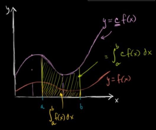
Integrating sums of functions
$$ \begin{gather} \int_a^b (f(x) \pm g(x)) dx = \int_a^b f(x) dx \pm \int_a^b g(x) dx\\ \end{gather} $$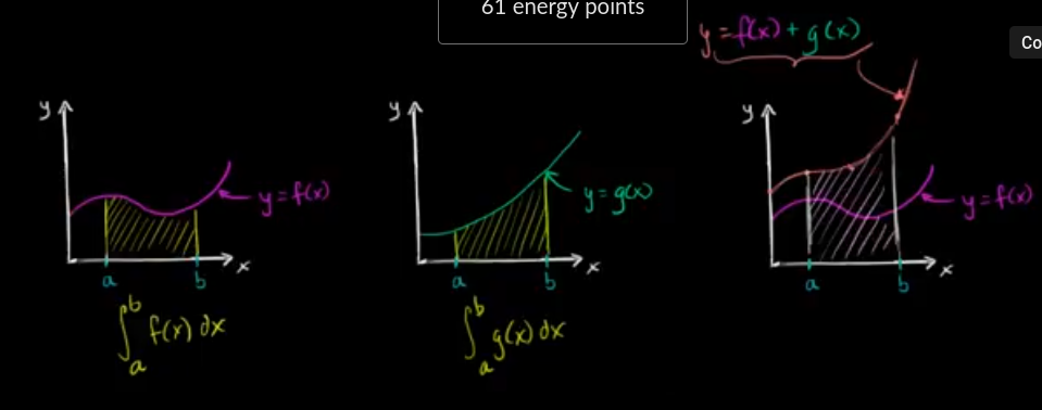
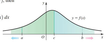
Definite integrals on adjacent intervals
$$ \begin{gather} \int_a^b f(x) dx = \int_a^c f(x) dx + \int_c^b f(x) dx\\ \end{gather} $$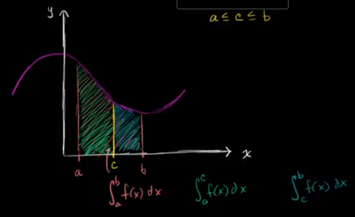
The function $|f|$ is integrable on $[a, b]$, and $\int_a^b |f(x)|dx$ is the sum of the areas of the regions bounded by the graph of $f$ and the x-axis on $[a, b]$.
$x$ on both bounds
Given
$$ \begin{gather} F(x) = \int_x^{x^2} f(t) dt \end{gather} $$We have:
$$ \begin{gather} F(x) = \int_x^C f(t) dt + \int_C^{x^2} f(t) dt\\ = \int_- C^x f(t) dt + \int_C^{x^2} f(t) dt\\ \end{gather} $$Evaluating Definite Integrals
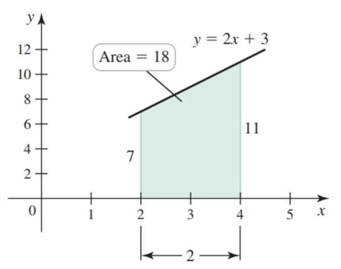
Evaluating Definite Integrals Using Geometry
Some definite integrals can be evaluated using geometry e.g. $\int_2^4 (2x + 3) dx$ is determined witht he formula of a trapezoid:
Evaluating Definite Integrals from Graphs
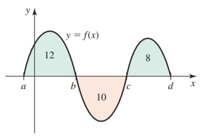
- $\int_a^b f(x) dx = 12$
- $\int_b^c f(x) dx = -10$
- $\int_a^c f(x) dx = 12 - 10 = 2$
Evaluting Definite Integrals Using Limits
For areas that cannot derived using the previous method we use a right Riemann sum letting $n \to \infty$
The formula for the definite integral we will use is:
$$ \begin{align} \lim_{n \to \infty} \sum_{k = 1}^n f(a + k \Delta x) \Delta x \end{align} $$We can solve the definite integral $\int_0^2 (x^3 + 1) dx$ with the following steps leaving $n$ unsubstituted until the end:
- Find $\Delta x = \frac{b - a}{n} = \frac{2 - 0}{n}$
- the right Riemann sum is
- We can substitute in $\sum_{k = 1}^n k^3$ for one of the known closed formulas:
- Now, we evaluate the limit as $n \to \infty$:
Example-001. Definite integral
Write the following definite integral as the limit of a Riemann sum.
$$ \begin{gather} \displaystyle \int_\pi^{2\pi} \cos(x)\,dx \end{gather} $$Find $\Delta x$:
$$ \begin{gather} \begin{aligned} \greenD{\Delta x}&=\dfrac{ b- a}{n} \\\\ &=\dfrac{{2\pi}- \pi}{n} \\\\ &=\greenD{\dfrac{\pi}{n}} \end{aligned} \end{gather} $$Now, we can find $x_i$:
$$ \begin{gather} \begin{aligned} \blueD{x_i}&= a+\greenD{\Delta x}\cdot i \\\\ &= \pi+\greenD{\dfrac{\pi}{n}}\cdot i \\\\ &=\blueD{\pi+\dfrac{\pi i}{n}} \end{aligned} \end{gather} $$Therefore,
$$ \begin{gather} \displaystyle \int_\pi^{2\pi} \cos(x)\,dx=\lim_{n\to\infty}\sum_{i=1}^n\greenD{\dfrac\pi n}\cdot \goldD{\cos\left(\blueD{\pi+\dfrac{\pi i}n}\right)} \end{gather} $$Example-002. Find the definite integral
What is a limit that is equivalent to the following definite integral:
$$ \begin{gather} \displaystyle \int_{-2}^3 (x+1)\,dx \end{gather} $$We find $\Delta x$:
$$ \begin{gather} \displaystyle \Delta x=\dfrac{b-a}n=\dfrac{3-(-2)}n=\dfrac{5}n\, \end{gather} $$The right Riemann sum with $n$ terms is:
$$ \begin{gather} \displaystyle \sum_{i=1}^n f(a+i\Delta x)\cdot \Delta x = \sum_{i=1}^n\left(\dfrac{5i}n-1\right)\cdot \dfrac{5}n \end{gather} $$Therefore, we have:
$$ \begin{gather} \displaystyle \int_{-2}^{3} (x+1)\,dx = \lim_{n\to\infty}\sum_{i=1}^n \left(\dfrac{5i}n-1\right)\cdot \dfrac{5}n \end{gather} $$Negative Definite Integrals
$$ \begin{gather} \int_c^c f(x) dx = 0 \end{gather} $$Area Functions
We can define a function using a definite integral:
$$ \begin{gather} g(x) = \int_{-2}^x f(t) dt \end{gather} $$And, here is a table with various values for $x$:
| $x$ | $g(x)$ |
|---|---|
| $1$ | $\int_{-2}^1 f(t)dt$ |
| $2$ | $\int_{-2}^2 f(t)dt$ |
| $3$ | $\int_{-2}^3 f(t)dt$ |
Table: Table-001. Definite integral that is a function of another function
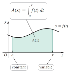
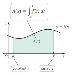
Given a continuous function $y = f(t)$ defined for $t \geq a$, where $a$ is a fixed number, the area function for $f$ with left endpoint $a$ is denoted $A(x)$. It gives the net area of the region bounded by the graph of $f$ and the $t$-axis between $t = a$ and $t = x$. The net area is also given by the definite integral:
$$ \begin{align} A(x) = \int_a^x f(t) dt \end{align} $$- Note that $x$ is the upper limit and the independent variable
Given the two area functions $A_1(x) = \int_{-1}^x f(t) dt$ and $A_2(x) = \int_3^x f(t) dt$ and results provided by the graph below, we make the following observations.
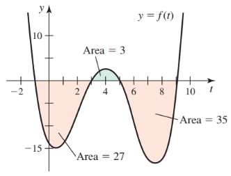
- $A(3) = -27, F(3) = 0; A(3) - F(3) = -27$
- $A(5) = -24, F(5) = 3; A(5) - F(5) = -27$
- $A(9) = -59, F(9) = -32; A(9) - F(9) = -27$
Given the trapezoid bounded by the line $f(t) = 2t + 3$ and the $t$-axis from $t = 2$ to $t = x$. The area function $A(x) = \int_2^x f(t) dt$ gives the area of the trapezoid, for $x \geq 2$.
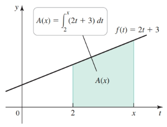
Given the formula for the area of a trapzoid of $A = \frac{1}{2}h(a + b)$ we can set up the following equality and find the result for the area:
$$ \begin{align} A(5) = \int_2^5 (2t + 3) dt = \frac{1}{2} (5 - 2) \cdot (f(2) + f(5))\\ = \frac{1}{2} \cdot 3 (7 + 13)\\ = 30 \end{align} $$Using $x$ instead as our right endpoint we have:
$$ \begin{align} A(x) = \frac{1}{2}(x - 2) \cdot (f(2) + f(x))\\ = \frac{1}{2}(x - 2)(7 + 2x + 3)\\ = x^2 + 3x - 10 \end{align} $$Expressing the $A(x)$ in terms of an integral with a variable upper limit gives us the following equality
$$ \begin{align} A(x) = \int_2^x (2t + 3)dt = x^2 + 3x - 10 \end{align} $$Differentiating $A(x)$ we find that:
$$ \begin{align} A'(x) = \frac{d}{dx}(x^2 + 3x - 10) = 2x + 3 = f(x) \end{align} $$Therefore, $A$ is an antiderivative of $f$. This leads to the Fundamental Theorem of Calculus.
Fundamental Theorem of Calculus: Part 1
If $f$ is continuous on $[a, b]$, then the area function:
$$ \begin{align} A(x) = \int_a^x f(t) dt, \text{ for } a \leq x \leq b \end{align} $$is continuous on $[a, b]$ and differentiable on $(a, b)$. The area function satisfies $A'(x) = f(x)$.
Equivalently,
$$ \begin{align} A'(x) = \frac{d}{dx} \underbrace{\int_a^x f(t)}_{A(x)} dt = f(x) \end{align} $$which means that the area function of $f$ is an antiderivative of $f$ on $[a, b]$.
Note that $A(x)$ and $F(x)$ are antiderivatives of $f(x)$ i.e. $A'(x) = F'(x) = f(x)$. That is we more or less take the antiderivative of a function and we have that function’s area equation.
Given the derivative of integral $\frac{d}{dx} \int_1^x \sin^2 t dt$ the following is true:
$$ \begin{align} \frac{d}{dx} \int_1^x \sin^2 t dt = \sin^2 x \end{align} $$Note the appropriate use of $t$ and $x$
In other words, if I have:
$$ \begin{gather} g(x) = \int_{19}^x \sqrt[3]{t} \end{gather} $$then, if I differentiate with respect to $x$ then I get the RHS as a function with respect to $t$:
$$ \begin{gather} \frac{d}{dx}[g(x)] = \frac{d}{dx}\left[\int_{19}^x \sqrt[3]{t} \right]\\ g'(x) = \sqrt[3]{x} \end{gather} $$Liebniz’s rule
$$ \begin{align} \frac{d}{dx} \int^{g(x)}_a f(t) dt = f(g(x)) g'(x) \end{align} $$We can evaluate the definite integral $\frac{d}{dx} \int_0^{x^2} \cos t^2 dt$ with the following steps:
- Since the upper limit of $x$ is a function of $x$, let $u = x^2$ to produce:
By the Chain Rule,
$$ \begin{align} \frac{d}{dx} \int_0^{x^2} dt = \frac{dy}{dx} = \frac{dy}{du} \frac{du}{dx}\\ = \left(\frac{d}{du} \int_0^u \cos t^2 dt\right)(2x)\\ = (\cos u^2)(2x)\\ = 2x \cos x^4 \end{align} $$Another Perspective
Let’s say we have:
$$ \begin{gather} F(x) = \int_{1}^{\sin(x)} (2t - 1) dt \end{gather} $$We have two functions on the RHS:
$$ \begin{gather} h(x) = \int_{1}^{x} (2t - 1) dt\\ g(x) = \sin(x) \end{gather} $$So,
$$ \begin{gather} F(x) = h(g(x)) \end{gather} $$The chain rule gives us:
$$ \begin{gather} F'(x) = h'(g(x)) \cdot g'(x) \end{gather} $$So,
$$ \begin{gather} F'(x) = (2(\sin(x)) - 1) \cdot \cos(x) \end{gather} $$Interpreting the Behavior of Accumulation Functions
In differential calculus we reasoned about the properties of a function $f$ based on information given about its derivative $'f$. In integral calculus, instead of talking about functions and their derivatives, we will talk about functions and their antiderivatives. We reason from $f'$ to $f$.
Consider the graph of function $f$
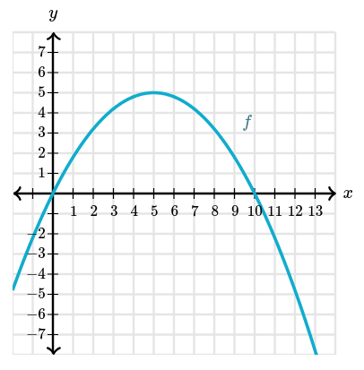
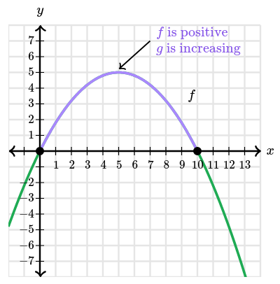
Let $g(x)=\displaystyle\int_0^x f(t)\,dt$. Defined this way, $g$ is an antiderivative of $f$. In differential calculus we would write this as $g' = f$. Since $f$ is the derivative of $g$, we can reason about properties of $g$ in similar to what we did in differential calculus. For example, $f$ is positive on the interval $[0, 10]$, so $g$ must be increasing on this interval.
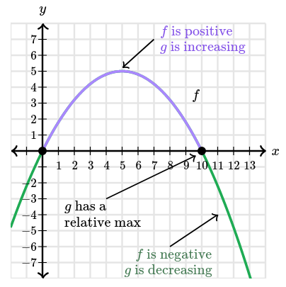
Furthermore, $f$ changes its sign at $x = 10$, so $g$ must have an extremum there. Since $f$ goes from positive to negative, that point must be a maximum point.
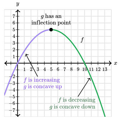
We can also reason about the concavity of $g$. Since $f$ is increasing on the interval $[-2, 5]$, we know $g$ is concave up on that interval. And since $f$ is decreasing on the interval $[5, 13]$, we know $g$ is concave down on that interval. $g$ changes concavity at $x = 5$, so it has an inflection point there.
Fundamental Theorem of Calculus: Part 2
Given the following:
$$ \begin{gather} F(x) = \int_{c}^x f(t) dt\\ F'(x) = f(x) \end{gather} $$The fundamental theorem of calculus also gives us the following:
$$ \begin{gather} F(b) - F(a) = \int_{c}^b f(t) dt - \int_{c}^a f(t) dt = \int_{a}^b f(t) dt, b \gt a\\ \end{gather} $$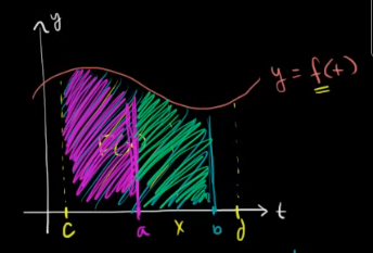
Further, if we take the derivative of this we get $0$ (since $F(b) - F(a)$ is a constant), i.e.:
$$ \begin{align} \frac{d}{dx} \int_a^b f(t) dt = 0 \end{align} $$It is customary to denote $F(b) - F(a)$ as
$$ \begin{align} F(x)|_a^b \end{align} $$OR
$$ \begin{align} [F(x)]_a^b \end{align} $$We can evaluate the definite integral $\int_0^{10} (60x - 6x^2) dx$ for the graph below with the following steps:
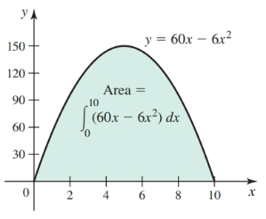
- First find the antiderivative of $60x - 6x^2$, $F(x) = 30x^2 - 2x^3$
- This leads us to the equation $(30x^2 - 2x^3)|_0^{10}$
- Next evaluate:
Piecewise Functions
$$ \begin{gather} f(x) = \begin{cases} \dfrac{5}{x} & \text{for} ~~~~x\gt{5} \\ x-4& \text{for} ~~~~ x \leq5\end{cases} \end{gather} $$Where for $f(x)$:
$$ \begin{gather} \displaystyle\int^6_{4}f(x)\,dx = \end{gather} $$We have:
$$ \begin{gather} \int_4^5 x - 4 dx + \int_5^6 \frac{5}{x} dx\\ = \frac{x^2}{2} - 4x |_4^5 + 5 \ln(x) |_5^6\\ = \frac{1}{2} + 5 \ln \left(\frac{6}{5} \right) \end{gather} $$[sin or cos problem example because these are confusing…]
Even and Odd functions
- there are shortcuts for evaluating definite integrals for odd and even functions
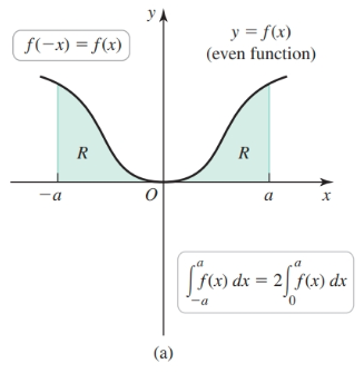
The following property holds for definite integrals of even functions:
$$ \begin{align} \int_{-a}^a f(x) dx = 2 \int_0^a f(x) dx \end{align} $$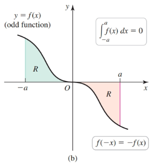
The following property holds for definite integrals of odd functions:
$$ \begin{align} \int_{-a}^a f(x) dx = 0 \end{align} $$Given a definite integral such as:
$$ \begin{align} \int_{-2}^2 (x^4 - 3x^3) dx \end{align} $$We can split the integral and then use symmetry:
$$ \begin{align} \int_{-2}^2 x^4 dx - 3 \int_{-2}^2 x^3 dx\\ = \frac{64}{5} - 0\\ = \frac{64}{5} \end{align} $$Average Value of a Function
The average value of an integrable function $f$ on the interval $[a, b]$ is
$$ \begin{align} \overline{f} = \frac{1}{b - a} \int_a^b f(x) dx \end{align} $$Multiplying both sides by $(b - a)$ gives us a the net area of a rectangle with that is equal to the net area of the region bounded by $f(x)$
$$ \begin{align} (b - a) \overline{f} = \int_a^b f(x) dx \end{align} $$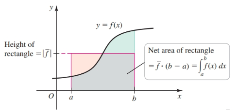
Mean Value Theorem for Integrals
Let $f$ be continuous on the interval $[a, b]$. There exists a point $c$ in $(a, b)$ such that
$$ \begin{align} f(c) = \overline{f} = \frac{1}{b - a} \int_a^b f(t) dt \end{align} $$[Find the $\overline{f}$, then solve for $c$ in $f(c) = \overline{f}$]
Substitution Rule with Indefinite Integrals and Definite Integrals
With certain integrals we can substitute parts of the variable of integration and parts of the integrand by finding an equation which is the derivative of an inner function or some component of the integrand.
Given the indefinite integral:
$$ \begin{align} \int f(g(x))g'(x) dx \end{align} $$Let $u = g(x)$:
$$ \begin{align} u = g(x)\\ du = g(x) dx \end{align} $$Now perform substitutions:
$$ \begin{align} \int f(u) du \end{align} $$With definite integral substitutions we must set our limits as a function of $u$:
$$ \begin{align} \int_a^b f(g(x))g'(x) dx = \int_{u(a)}^{u(b)} f(u) du \end{align} $$Some definite integrals can be solved with the use of substitution.
- Given an indefinite integral involving a composite function $f(g(x))$, identify the inner function $u = g(x)$ such that a constant multiple of $g'(x)$ appears in the integrand.
Given
$$ \begin{align} \int 2(2x + 1)^3 dx \end{align} $$We let $u = 2x + 1$ and find the derivative, expressing the equality with a side that can be substituted back into the original equation:
$$ \begin{align} \frac{du}{dx} = 2\\ du = 2 dx\\ \end{align} $$- Substitute $u = g(x)$ and $du = g'(x) dx$ in the integral.
The original equation becomes:
$$ \begin{align} \int u^3 du \end{align} $$- Evaluate the new indefinite integral with respect to $u$.
- Write the result in terms of $x$ using $u = g(x)$.
If the integral is a definite integral. Then there are additional steps.
Given that
Let $u = g(x)$, where $g'$ is continuous on $[a, b]$, and let $f$ be continuous on the range of $g$. Then
$$ \begin{align} \int_a^b f(g(x)) g'(x) dx = \int_{g(a)}^{g(b)} f(u) du \end{align} $$You may find the solution by using the Fundamental Theorem of Calculus and evaluating $F(b) - F(a)$.
Another more efficient method is to change the limits of integration and complete the integration with respect to $u$.
Given $\int_0^2 \frac{dx}{(x + 3)^3}$
Let the new variable be $u = x + 3$ and then $du = dx$.
We have
$$ \begin{align} \int_3^5 u^{-3} du \end{align} $$We can use the equation for $u$ to find the new limits:
$$ \begin{align} \frac{u^{-2}}{2}|_3^5\\ = -\frac{1}{2} (5^{-2} - 3^{-2})\\ = \frac{8}{225} \end{align} $$Using Substitution to Find Indefinite Integrals
Given $\int f(g(x)) dx$ e.g. $\int (3x + 1)^{10} dx$
- Substitute $u$ for $g(x)$ i.e. $\int u^{10} dx, u = 3x + 1$
- Find the derivative of $u$ with respect to $x$ e.g. $\frac{du}{dx} = 3$
- Express this equation in terms of $dx$ e.g. $dx = \frac{du}{3}$
- Substitute $dx$ in terms of $du$ into the indefinite integral expression e.g. $\int u^{10} \frac{du}{3} = \frac{1}{3} \int u^{10} \: du$
- Solve, leaving $du$ behind e.g. $\frac{1}{3} \frac{u^{11}}{11} + C$
- Substitute $g(x)$ for $u$ e.g. $\frac{1}{3} \frac{(3x + 1)^11}{11} + C = \frac{(3x + 1)^11}{33} + C$
- Check by finding the derivative of the result.
Given another problem you can end up with an expression containing a term in the original function and $dx$ and be able to substitute both back in:
$$ \begin{align} \int x^4 e^{2x^5 + 13}dx\\ \end{align} $$Assign a $u$:
$$ \begin{align} u = 2x^5 + 13\\ \frac{du}{dx} = 10x^4\\ \frac{1}{10} du = x^4 dx\\ \end{align} $$We are able to substitute $x^4$ and $dx$ for $\frac{1}{10}$ and $du$
$$ \begin{align} \frac{1}{10} \int e^4 du\\ \frac{1}{10} e^{2x^5 + 13} + C \end{align} $$pg 388
Given rational function such that the numerator is $1$ degree less then the denominator, a $u$ substitution can be easily performed:
$$ \begin{align} \int \frac{x^{99}}{x^{100}} dx\\ \end{align} $$Substitute the denominator:
$$ \begin{align} u = x^{100}\\ du = 100x^{99} dx\\ \frac{du}{100} = x^{99} dx \end{align} $$Substitute $u$ and $du$ in:
$$ \begin{align} \int \frac{1}{100 u} du \end{align} $$More exotic substitutions:
$$ \begin{align} \int x^2 \tan^{-1}(10x) dx\\ \end{align} $$$$ \begin{align} u = 10x\\ du = 10 dx\\ \frac{du}{10} = dx \end{align} $$This means that $x = \frac{u}{10}$:
$$ \begin{align} \int \frac{u^2}{10} \tan^{-1}{u} \frac{1}{10} du \end{align} $$Some substitutions can be especially tricky:
$$ \begin{align} \int \frac{\sqrt{x - 3}}{x} dx \end{align} $$This an awkward subsitution:
$$ \begin{align} u = \sqrt{x - 3}\\ = (x - 3)^{\frac{1}{2}}\\ du = \frac{1}{2} (x - 3)^{-\frac{1}{2}}\\ \frac{1}{2\sqrt{x - 3}} dx\\ 2\sqrt{x - 3} du = dx \end{align} $$We partially substitute back in:
$$ \begin{align} \int \frac{2 \sqrt{x - 3} \sqrt{x - 3}}{x} du\\ \int \frac{2(x - 3)}{x} du\\ \end{align} $$$$ \begin{align} u = \sqrt{x - 3}\\ u^2 = x - 3\\ u^2 + 3 = x \end{align} $$Finally, we have (which can be solved by trigonometric substitution):
$$ \begin{align} \int \frac{2u^2}{u^2 + 3} du \end{align} $$Given the problem:
$$ \begin{align} \int \frac{t^3 + 4}{t^4 + 16t + 8} dt \end{align} $$We use the following substitution:
$$ \begin{align} u = t^4 + 16t + 8\\ du = (4t^3 + 16)dt\\ du = 4(t^3 + 4)dt\\ \frac{du}{4} = (t^3 + 4)dt\\ \end{align} $$Observe how the substitution works when there are two operands in the derivative on the RHS.
It may be the case that you can split up in the integral and perform a substitution on just one operand:
$$ \begin{align} \int \tan^4 8t dt\\ = \int \tan^2 8t \tan^2 8t dt\\ = \int \tan^2 8t (sec^2 8t - 1) dt\\ = \int \tan^2 8t sec^2 8t - \tan^2 dt\\ = \int \tan^2 8t sec^2 8t dt - \int \tan^2 dt \end{align} $$We can now perform a substitution on the first term while leaving the second term alone:
$$ \begin{align} u = \tan 8t\\ du = 8 \sec^2 8t dt\\ \frac{du}{8} = \sec^2 8t dt \end{align} $$Substituting back in we have:
$$ \begin{align} \int \tan^2 8t sec^2 8t dt - \int \tan^2 dt \end{align} $$Strategies for Solving Integrals
$$ \begin{align} -2 \int_1^0 f(x) dx = 2 \int_0^1 f(x) dx\\ \int_0^1 \sqrt{x} dx = \int_0^1 x^{\frac{1}{2}} dx\\ \int \frac{1}{x^{n} dx = \int x^{-n} dx, |n| \ne 1 \end{align} $$Look for trigonometric substitutions:
$$ \begin{align} \int \sin x \sec x dx\\ \int \frac{\sin x}{\cos x} dx\\ \end{align} $$Regions Between Curves
- the region between two curves is solved using the slice and sum strategy used for Riemann sums
- the following formula approximates area:
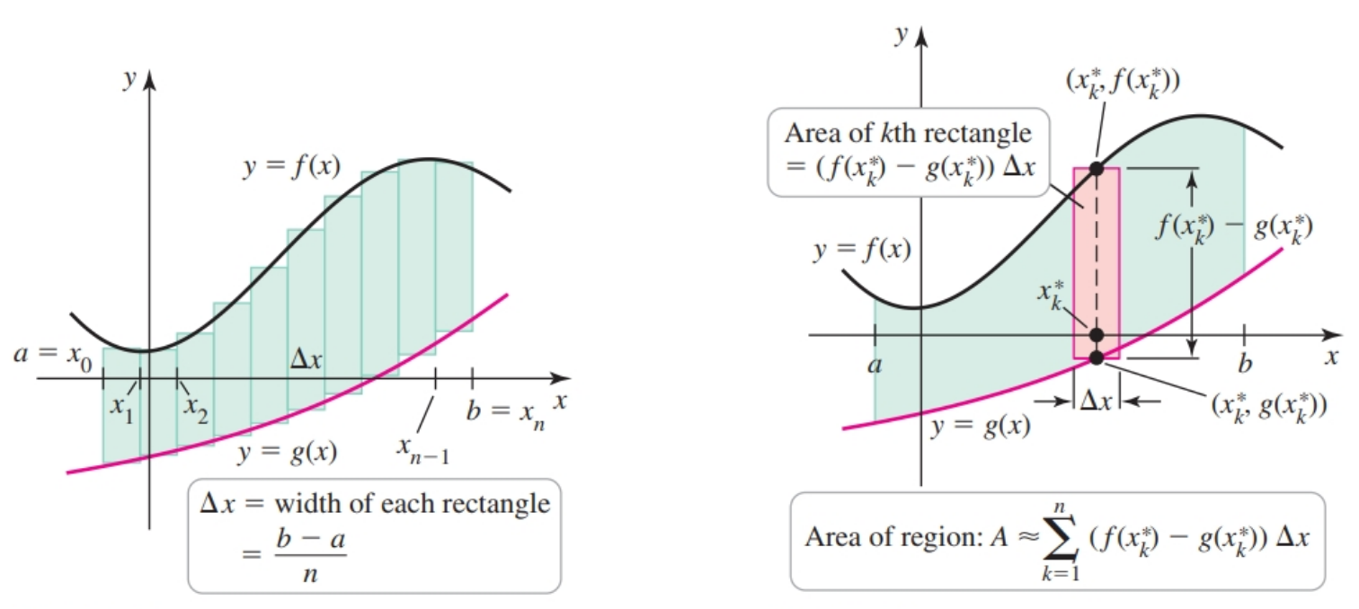
As the number of grid points increases, $\Delta x$ approaches zero and these sums approach the area of the region between the curves; that is,
$$ \begin{align} A = \lim_{n \to \infty} \sum_{k = 1}^n (f(x_k^*) - g(x_k^*)) \Delta x \end{align} $$The area can also be expressed with definite integrals:
$$ \begin{align} A = \int_a^b (f(x) - g(x)) dx \end{align} $$Integrating with Respect to y
- sometimes it makes more sense to solve with respect to $y$
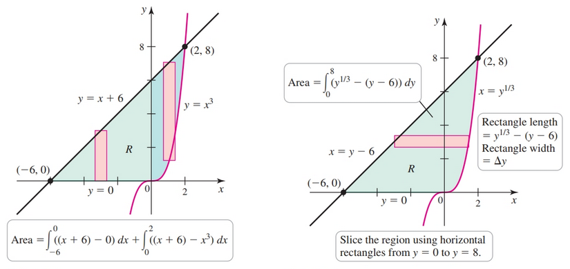
In such cases, we treat $y$ as the independent variable and divide the interval $[c, d]$ into $n$ subintervals of width $\Delta y = (d - c)/n$. On the $k$th subinterval, a point $y_k^*$ is selected, and we construct a rectangle that extends from the left curve to the right curve. The $k$th rectangle has length $f(y_k^*) - g(y_k^*)$, so the area of the $k$th rectangle is $(f(y_k^*) - g(y_k^*)) \Delta y$. The area of the region is approximated by the sum of the areas of the rectangles.
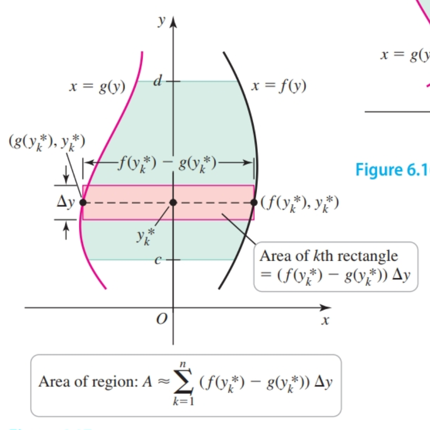
In the limit as $n \to \infty$ and $\Delta y \to 0$, the area of the region is given as the definite integral:
$$ \begin{align} A = \lim_{n \to \infty} \sum_{k = 1}^n (f(y_k^*) - g(y_k^*)) \Delta y\\ = \int_c^d (f(y) - g(y))dy \end{align} $$Volumes of Solids
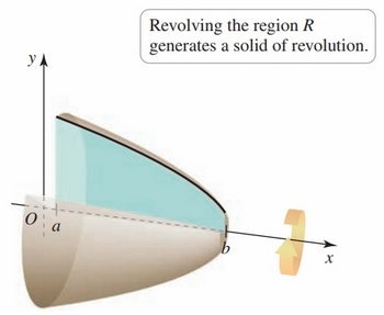
Revolving a region around some axis e.g. y-axis, x-axis, x = 4, etc. results in a solid of revolution.
The Riemann sum slice and sum strategy is fundamental to finding these volumes.
The Disk Method
- Some solids of revolution allow us to “slice” and “sum” disk-like objects.
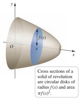
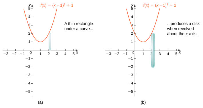
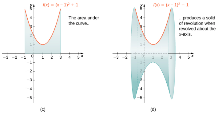
The formula for volume of a disk in lay terms is:
$$ \begin{align} \pi (\text{radius})^2 (\text{thickness}) \end{align} $$Where the radius is given by the function and the thickness is the $x$ differential.
The area of a given disk at point $x$, where $a \leq x \leq b$, is given by the function:
$$ \begin{align} A(x) = \pi(\text{radius})^2 = \pi f^2(x) \end{align} $$The volume of a typical rectangle is given by:
$$ \begin{align} \Delta V = \pi f^2(x) \Delta x \end{align} $$By the general slicing method, the volume of the solid is
$$ \begin{align} V = \int_a^b A(x) dx = \int_a^b \pi f(x)^2 dx \end{align} $$The limits of integration are the bounds of the region parallel to the faces of the disk.
The Washer Method
- Some solids of revolution allow us to “slice” and “sum” washer-like objects:
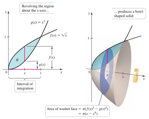
In lay terms, the formula for a washer is:
$$ \begin{align} \pi [ (\text{outer radius})^2 - (\text{inner radius})^2 ] (\text{thickness}) \end{align} $$The formula for the volume of a typical washer is:
$$ \begin{align} V(x) = \pi [ f^2(x) - g^2(x) ] \Delta x \end{align} $$The formula for the exact volume of the solid is:
$$ \begin{align} V = \int_a^b \pi(f(x)^2 - g(x)^2) dx \end{align} $$The limits of integration are the bounds of the region parallel to the faces of the washer.
Revolving About the y-axis
- We can revolve about the $y$-axis as well
- rewrite the functions in terms of $y$
Washer Method example
$$ \begin{align} V = \int_c^d \pi(p(y)^2 - q(y)^2)dy \end{align} $$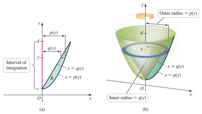
Shell Method
Some revolution solids are more easily computed with the shell method wherein the sums are the result of many concentric cylinders:
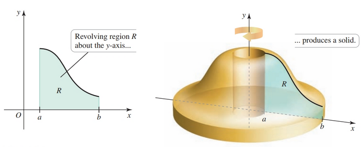
To solve this volume using the disk method, we would utilize cross-sections perpendicular to the axis of revolution. (The direction of the cross sections is one difference). Instead, we utilize cross-sections vertical to the axis of revolution.
In lay terms the volume of a typical cylinder of the shell is:
$$ \begin{align} \Delta V = \pi \overbrace{2 (\frac{\text{outer radius} + \text{inner radius}}{2})}^{\text{gives average radius}} \cdot \text{height} \cdot \overbrace{(\text{outer radius} - \text{inner radius})}^{\text{thickness}}\\ = \pi 2 r h \Delta r \end{align} $$This in turn results in the volume formula:
$$ \begin{align} V = \int_a^b \pi 2 x \overbrace{(f(x) - g(x))}^{\text{height}} \overbrace{dx}^{\text{thickness}} \end{align} $$Strategies for Solving Revolution Solids
A definite integral of symmetric even functions can be rewritten:
$$ \begin{align} \int_{-a}^a (f_1(x)^{\text{even number}} + f_2(x)^{\text{even number}} + \dots + f_n(x)^{\text{even number}}) dx\\ = 2 \int_{0}^a (f_1(x)^{\text{even number}} + f_2(x)^{\text{even number}} + \dots + f_n(x)^{\text{even number}}) dx\\ \end{align} $$Depending on the method and axis of revolution, it may make more sense to solve in terms of $y$. Given $y = f(x)$, find $x = g(y)$, and update the integral accordingly:
$$ \begin{align} V = \int_{f(a)}^{f(b)} A(y) dy \end{align} $$In some cases it may make sense to use a different method e.g. washer method instead of shell method.
Substitute trigonometric identities when it makes sense.
Revolving About Other Axes
It may be the case that you are not revolving about the $x$- or $y$-axis, but some other axis. In that case the formulas must be adjusted accordingly. Below the adjustments are shown for revolutions about the $x$-axis, but are applicable to revolutions about the $y$-axis as well.
Consider the importance of the distance from a given axis in determining area, and not Cartesian values.
If $a \lt b \leq c$ then we must subtract out values from the axis of revolution.
For the disk method we have:
$$ \begin{align} V = \pi \int_a^b (c - f(x))^2 dx \end{align} $$For the washer method we have (where $f(x) \geq g(x), \text{ for all }x, a \leq x \leq b$):
$$ \begin{align} V = \pi \int_a^b [(c - g(x)) - (c - f(x))]^2 dx \end{align} $$- Note the change in position of $f(x)$ and $g(x)$
For the shell method (where $f(y) \geq g(y), \text{ for all }y, a \leq y \leq b \$):
$$ \begin{align} V = 2 \pi \int_a^b (c - y)[f(y) - g(y)]^2 dy \end{align} $$If $c \leq a \lt b$ then we must subtract $c$.
For the disk method we have:
$$ \begin{align} V = \pi \int_a^b (f(x) - c)^2 dx \end{align} $$For the washer method we have (where $f(x) \geq g(x), \text{ for all }x, a \leq x \leq b$):
$$ \begin{align} V = \pi \int_a^b [(f(x) - c) - (g(x) - c)]^2 dx \end{align} $$- Recall that subtracting a negative results in a difference that is larger than the operands.
For the shell method (where $f(y) \geq g(y), \text{ for all }y, a \leq y \leq b \$):
$$ \begin{align} V = 2 \pi \int_a^b (y - c)[f(y) - g(y)]^2 dy \end{align} $$Arc Length
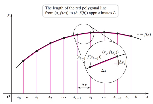
We divide $[a, b]$ into $n$ subintervals of length $\Delta x = (b - a)/n$, $x_k$ is the right endpoint of the $k$th subinterval, for $k = 1, \dots, n$. Joining the corresponding points on the curve by line segments, we obtain a polygonal line with $n$ line segments. If $n$ is large and $\Delta x$ is small, the length of the polygonal line is a good approximation to the length of the actual curve. The strategy is to find the length of the polygonal line and then let $n$ increase, while $\Delta x$ goes to zero, to get the exact length of the curve.
Consider the $k$th subinterval $[x_{k - 1}, x_k]$ and the line segment between the points $(x_{k - 1}, f(x_{k - 1}))$ and $(x_k, f(x_k))$. We have the change in the $y$-coordinate and change $x$-coordinate as:
$$ \begin{align} \Delta y_k = f(x_k) - f(x_{k - 1})\\ \Delta x_k = x_k - x_{k - 1} \end{align} $$Knowing the formula for distance between two points we can find the length of segment $k$ with:
$$ \begin{align} \sqrt{(\Delta x)^2 + |\Delta y_k|^2}, \text{ for } k = 1, 2, \dots, n \end{align} $$Summing these lengths, we obtain the length of the polygonal line, which approximates the length $L$ of the curve:
$$ \begin{align} L \approx \sum_{k = 1}^n \sqrt{(\Delta x)^2 + |\Delta y_k|^2} \end{align} $$
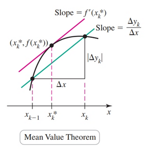
Since we have two terms $x$ and $y$, we cannot yet find the limit. Note that the slope of the $k$th subinterval is $\frac{\Delta y_k}{\Delta x}$. By mean value theorem this slope equals $f'(x_k^*)$ for some point $x_k^*$ on the $k$th subinterval.
Therefore,
$$ \begin{align} L \approx \sum_{k = 1}^n \sqrt{(\Delta x)^2 + |\Delta y_k|^2}\\ \end{align} $$Factor out $(\Delta x)^2$:
$$ \begin{align} = \sum_{k = 1}^n \sqrt{(\Delta x)^2 \left(1 + \left(\frac{\Delta y_k}{\Delta x}\right)^2\right)} \end{align} $$Bring $\Delta x$ out of the square root:
$$ \begin{align} = \sum_{k = 1}^n \sqrt{1 + \left(\frac{\Delta y_k}{\Delta x}\right)^2} \Delta x \end{align} $$Mean Value Theorem:
$$ \begin{align} = \sum_{k = 1}^n \sqrt{1 + f'(x_k^*)^2} \Delta x \end{align} $$Now we have a Riemann sum. As $n$ increases and as $\Delta x$ approaches zero, the sum approaches a definite integral, which is also the exact length of the curve. We have:
$$ \begin{align} L = \lim_{n \to \infty} \sum_{k = 1}^n \sqrt{1 + f'(x_k^*)^2} \Delta x\\ = \int_a^b \sqrt{1 + f'(x)^2} dx \end{align} $$A curve may be defined paramatrically e.g. $x = g(t), y = g(t)$. In that case we use similar reasoning to arrive at the following formula:
$$ \begin{align} L = \int_a^b \sqrt{\left(\frac{dx}{dt}\right)^2 + \left(\frac{dy}{dt}\right)^2} dt \end{align} $$Given a curve in terms of $x = f(t), y = g(t)$, simply find their derivatives and plug them into the formula.
We can also treat this as a general formula and reason backwards. If the curve is given in terms of $x$ we can substitute $dt$ for $dx$ and plug in the derivative of $y = f(x)$ ($\frac{dy}{dx}$):
$$ \begin{align} L = \int_a^b \sqrt{\left(\frac{dx}{dx}\right)^2 + \left(\frac{dy}{dx}\right)^2} dx\\ = \int_a^b \sqrt{1 + \left(\frac{dy}{dx}\right)^2} dx \end{align} $$If the curve is given in terms of $y$ we can substitute $dt$ for $dy$ and plug in the derivative of $x = f(y)$ ($\frac{dx}{dy}$):
$$ \begin{align} L = \int_a^b \sqrt{\left(\frac{dx}{dy}\right)^2 + \left(\frac{dy}{dy}\right)^2} dx\\ = \int_a^b \sqrt{\left(\frac{dx}{dy}\right)^2 + 1} dx \end{align} $$Strategies
Given a Cartesian formula we can always rewrite the equation in terms of the other variable. Given $y = f(x)$, first find $x = g(y)$ and update the limits of integration:
$$ \begin{align} \int_{f(a)}^{f(b)} \sqrt{1 + [g'(y)]^2} dy \end{align} $$Surface Area
- surface area calculations are “between” volume problems and arc length problems
Finding the surface area of a frustrum illustrates the intuition behind these types of problems:
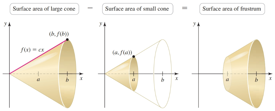
We will use a similar technique to find the surface area of a revoution.
We begin by dividing the interval $[a, b]$ into $n$ subintervals of equal length $\Delta x = \frac{b - a}{n}$.
The grid points in this partition are
$$ \begin{align} x_0 = a, x_1, x_2, \dots, x_{n - 1}, x_n = b \end{align} $$Now consider the $k$th subinterval $[x_{k - 1}, x_k]$ and the line segment betwee the points $(x_{k - 1}, f(x_{k - 1}))$ and $(x_k, f(x_k))$. We let the change in the $y$-coordinates between these points be $\Delta y = f(x_k) - f(x_{k - 1})$.
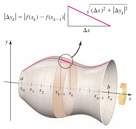
When this line segment is revolved about the x-axis, it generates a frustum of a cone. The slant height of this frustum is the length of the hypotenuse of a right triangle whose sides have lengths $\Delta x$ and $\Delta y$. Therefore, the slant height of the $k$th frustum is
$$ \begin{align} \sqrt{(\Delta x)^2 + | \Delta y_k|^2}\\ = \sqrt{(\Delta x)^2 + (\Delta y_k)^2} \end{align} $$and its surface area is
$$ \begin{align} S_k = \pi(f(x_k) + f(x_{k - 1})) \sqrt{(\Delta x)^2 + (\Delta y_k)^2} \end{align} $$It follows that the area $S$ of the entire surface of revolution is approximately the sum of the surface areas of the individual frustums $S_k$, for $k = 1, \dots, n$; that is,
$$ \begin{align} S \approx \sum_{k = 1}^n S_k = \sum_{k = 1}^n \pi(f(x_k) + f(x_{k - 1})) \sqrt{(\Delta x)^2 + (\Delta y_k)^2} \end{align} $$We apply the Mean Value Theorem on the $k$th subinterval $[x_{k - 1}, x_k]$ and observe that
$$ \begin{align} \frac{f(x_k) - f(x_{k - 1})}{\Delta x} = f'(x_k^*) \end{align} $$for some number $x_k^*$ in the interval $(x_{k - 1}, x_k)$, for $k = 1, \dots, n$. It follows that $\Delta y_k = f(x_k) - f(x_{k - 1}) = f'(x_k^*) \Delta x$.
We now replace $\Delta y_k$ with $f'(x_k^*) \Delta x$ in the expression for the approximate surface area. The result is
$$ \begin{align} S \approx \sum_{k = 1}^n S_k = \sum_{k = 1}^n \pi(f(x_k) + f(x_{k - 1}) \sqrt{(\Delta x)^2 + (\Delta y_k)^2} \end{align} $$Mean Value Theorem:
$$ \begin{align} = \sum_{k = 1}^n \pi(f(x_k) + f(x_{k - 1})) \sqrt{(\Delta x)^2(1 + f'(x_k^*)^2 \end{align} $$Factor out $\Delta x$:
$$ \begin{align} = \sum_{k = 1}^n \pi(f(x_k) + f(x_{k - 1})) \sqrt{1 + f'(x_k^*)^2} \Delta x \end{align} $$When $\Delta x$ is small, we have $x_{k - 1} \approx x_k \approx x_k^*$, and by continuity of $f$, it follows that $f(x_{k - 1}) \approx f(x_k) \approx f(x_k^*)$, for $k = 1, \dots, n$. These observations allow us to write
$$ \begin{align} SA \approx \sum_{k = 1}^n \pi(f(x_k^*) + f(x_k^*)) \sqrt{1 + f'(x_k^*)^2} \Delta x\\ = \sum_{k = 1}^n 2 \pi f(x_k^*) \sqrt{1 + f'(x_k^*)^2} \Delta x \end{align} $$This approximation to $S$, which has the form of a Riemann sum, improves as the number of subintervals increases and as the length of the subintervals approaches $0$. Specifically, as $n \to \infty$ and as $\Delta x \to 0$, we obtain an integral for the surface area:
$$ \begin{align} SA = \lim_{n \to \infty} \sum_{k = 1}^n 2 \pi f(x_k^*) \sqrt{1 + f'(x_k^*)^2} \Delta x\\ = \int_a^b 2 \pi f(x) \sqrt{1 + f'(x)^2} dx\\ = 2 \pi \int_a^b f(x) \sqrt{1 + \left(\frac{dy}{dx}\right)^2} dx \end{align} $$- Recall that we are revolving about the $x$-axis
- Note that $a$ and $b$ are $x$-values, and our differential is $dx$ and our derivative $\frac{dy}{dx}$
- Additionally note that $f(x)$ gives a $y$-value
If we are revolving about the $y$-axis then a general formula is:
$$ \begin{align} SA = 2 \pi \int_c^d g(y) \sqrt{1 + \left(\frac{dx}{dy}\right)^2} dy \end{align} $$- Here $c$ and $d$ are $y$-values, and our differential is $dy$ and our derivative $\frac{dx}{dy}$
- Additionally note that $g(y)$ gives an $x$-value
Observe that if we are revolving about the $y$-axis the term outside of the square root gives an $x$ value. And, if we are revolving about the $x$-axis the term outside of the square root gives a $y$ value.
If our curve is parametric and we are given $x = f(t)$ and $y = g(t)$, a \leq t \leq b$, then our formula for revolving about the $x$-axis is:
$$ \begin{align} SA = 2 \pi \int_a^b g(t) \sqrt{\left(\frac{dx}{dt}\right)^2 + \left(\frac{dy}{dt}\right)^2} dt \end{align} $$Strategies for Solving Surface Area
It is possible to take an equation and rewrite in terms of the other variable. Given $y = f(x)$ and $g(y) = x$ and $a \leq x \leq b$ and revolving about the $x$-axis we have:
$$ \begin{align} SA = 2 \pi \int_a^b f(x) \sqrt{1 + \left(\frac{dy}{dx}\right)} dx \end{align} $$Which is equivalent to:
$$ \begin{align} SA = 2 \pi \int_{f(a)}^{f(b)} y \sqrt{1 + \left(\frac{dx}{dy}\right)} dy \end{align} $$- Note that we are now in terms of $y$ so just $y$ is outside the square root.
It can be easiest to derive the equation based on how $a$ and $b$ are expressed. For instance, given $f(x)$ if $a$ and $b$ are in terms of $y$ and you are revolving about the $x$-axis then find $g(y) = x$ and differentiate in terms of $y$:
$$ \begin{align} SA = 2 \pi \int_a^b y \sqrt{1 + \left(\frac{dx}{dy}\right)} dy \end{align} $$If you are instead revolving about the $y$-axis, you can still differentiate in terms of $y$, but now the term outside the square root needs to give an $x$ value:
$$ \begin{align} SA = 2 \pi \int_a^b g(y) \sqrt{1 + \left(\frac{dx}{dy} \right)} dy \end{align} $$Observe that the rest of the equation is fairly flexible, but if revolving about the $y$-axis the outside term gives an $x$ value, and if revolving about the $x$-axis the outside term gives a $y$ value.
Integration by Parts
The product rule states that:
$$ \begin{align} \frac{d}{dx}[f(x) \cdot g(x)] = f(x) g'(x) + g(x) f'(x) \end{align} $$We can express this in terms of indefinite integrals this way:
$$ \begin{align} u(x)v(x) = \int (u'(x) v(x) + u(x)v'(x)) dx\\ = \int u'(x) v(x) dx + \int u(x) v'(x) dx \end{align} $$We can rearrange this expression to get:
$$ \begin{align} \int u(x) \underbrace{v'(x) dx}_{dv} = u(x)v(x) - \int v(x) \underbrace{u'(x) dx}_{du} \end{align} $$which is the basic relationship for integration by parts. Noting that:
$$ \begin{align} \frac{du}{dx} = u'(x)\\ du = u'(x) dx \end{align} $$and
$$ \begin{align} \frac{dv}{dx} = v'(x)\\ dv = v'(x) dx \end{align} $$and suppressing the independent variable $x$ we have:
$$ \begin{align} \int u dv = uv - \int v du \end{align} $$Strategies
Given an integral such as $\int f(x) g(x) dx$ we must decide which term is easier to differentiate and which term is easier to integrate.
Given $\int x \sin x dx$, we can differentiate $x$, so we have $u = x, du = dx$; and integrate $\sin x dx$, so we have $dv = \sin x dx, v = -\cos x$:
$$ \begin{align} \int x \sin x dx = x \cos x - \int -\cos x dx + C\\ = \int x \sin x dx = x \cos x + \int \cos x dx + C \end{align} $$If we have one term we can integrate on $dx$. Given $\int \ln x dx$, we can differentiate $\ln x$, so we have $u = \ln x, du = \frac{1}{x}dx$; and integrate $dx$, so we have $dv = dx, v = x$:
$$ \begin{align} \int \ln x dx = x \ln x - \int x \frac{1}{2}dx \end{align} $$Definite Integrals
We modify the general formula slightly:
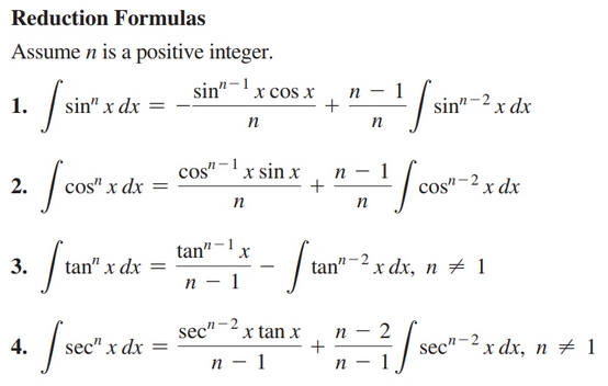
$$ \begin{align} \int_a^b u dv = uv|_a^b - \int_a^b v du \end{align} $$Trigonometric Integrals
- use trigonometric identities to solve trigonometric integrals
Given an integral such as:
$$ \begin{align} \int \sin^{ab} x dx \end{align} $$If $ab$ is odd we can split off a single $\sin x$:
$$ \begin{align} \int \sin x \sin^{ab - 1} x dx \end{align} $$Next, we substitute $\sin^{ab - 1} x$ with a Pythagorean identity:
$$ \begin{align} \int \sin x (1 - \cos^2 x)^{ab - 3} dx \end{align} $$Next, perform a substitution of $\cos^2 x$:
$$ \begin{align} u = \cos x\\ \frac{du}{dx} = -\sin x\\ du = \sin x dx\\ \end{align} $$Now, substitute $u$ and $-du$ back in (we also make the substitution $ab - 3 = 2$ to simplify things):
$$ \begin{align} -\int (1 - u^2)^{2} du\\ \end{align} $$Expand and solve:
$$ \begin{align} -\int u^4 - 2u^2 + 1 du\\ \dots\\ \frac{1}{5}u^5 - \frac{2}{3}u^3 + u + C \end{align} $$Finally, substitute $\cos x$ back in:
$$ \begin{align} \frac{1}{5} \cos^5 x - \frac{2}{3} \cos^3x + \cos x + C \end{align} $$Problems involving $\cos^{ab} x$ are solved similarly, e.g.:
$$ \begin{align} \int \cos^{ab} x dx \end{align} $$Integrating Products of Powers of $\sin x$ and $\cos x$, Powers of $\tan x$ and $\sec x$
When both $m$ and $n$ are even in an equation of the form:
$$ \begin{align} \int \sin^m x \cos^n x dx \end{align} $$We can perform the following substitutions using the half-angle identities (let $m = 2, n = 2$):
$$ \begin{align} \int \left[\frac{1}{2}(1 + \cos 2x)\frac{1}{2}(1 - \cos 2x)\right] dx \end{align} $$From here, we expand, perform a $u$ substitution, and integrate.
If $m$ is odd and $m > 1$ while $n$ is even in the form:
$$ \begin{align} \int \sin^m x \cos^n x dx \end{align} $$Factor out a $\sin x$:
$$ \begin{align} \int \sin^{m - 1} \cos^n \sin x dx \end{align} $$Perform the substitution $u = \cos x$ and this will eliminate $\sin x dx$.
If $n$ is odd and $n > 1$ while $m$ is even in the form:
$$ \begin{align} \int \sin^m x \cos^n x dx \end{align} $$Factor out a $\cos x$:
$$ \begin{align} \int \sin^{m} \cos^{n - 1} \cos x dx \end{align} $$Perform the substitution $u = \sin x$ and this will eliminate $\sin x dx$.
We can use similar techniques on problems of the form:
$$ \begin{align} \int \tan^m x \sec^n x \end{align} $$If $n$ is even then split off $sec^2 x$, rewrite the remaining even power of $\sec x$ in terms of $\tan x$, and use $u = \tan x$.
If $m$ is odd split off $\sec tan x$, rewrite the reamining even power of $\tan x$ in terms of $\sec x$, and use $u = \sec x$.
If $m$ is even and $n$ is odd rewrite the even power of $\tan x$ in terms of $\sec x$ to produce a polynomial in $\sec x$; apply the appropriate reduction formula to each term.
Table of Integrals
You can use a table of integrals to solve some integrals that have a specific form e.g. $\int \sin^8 x dx$
Strategies
Substitutions may need to be performed to make equations more amenable to a formula in the table of integrals.
In the following formula the argument to $\tan^{-1}$ must be a variable:
$$ \begin{align} \int x^2 \tan^{-1} 14x dx \end{align} $$So we perform a substitution:
$$ \begin{align} u = 14x\\ du = 14 dx\\ \frac{du}{14} = dx \end{align} $$Now, we have:
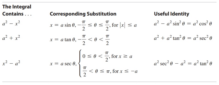
$$ \begin{align} \frac{1}{14^3} \int {u^2} \tan^{-1} u du \end{align} $$Trigonometric Substitutions
Right triangles and Pythagorean identities can be used to solve integrals that contain sums of squares and differences of squares of certain forms.
If we have an integral of the form $\int \frac{dx}{\sqrt{x^2 + a^2}}$ ($a$ is some constant) we can treat $\sqrt{x^2 + a^2}$ as the side of a right triangle:
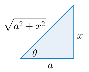
Further, since $\tan \theta = \frac{x}{a}$ we can derive the equation:
$$ \begin{align} x = a \tan \theta \end{align} $$We need to get rid of the $x$ so we differentitate this to find a substitute for $dx$:
$$ \begin{align} dx = a \sec^2 \theta d \theta \end{align} $$Now, we can substitute for $x$ in the original equation:
$$ \begin{align} \int \frac{a \sec^2 \theta d \theta}{\sqrt{a \tan^2 \theta + a^2}}\\ \end{align} $$$$ \begin{align} \int \frac{a \sec^2 \theta d}{\sqrt{a (\tan^2 \theta + 1)}}\\ \end{align} $$Now, substitute with the appropriate Pythagorean identity and solve:
$$ \begin{align} \int \frac{a \sec^2 \theta d \theta}{a \sec \theta}\\ = \int \sec \theta d \theta\\ = \ln |\sec \theta + \tan \theta| + C \end{align} $$Now, we use our triangle to substitute our $\theta$ in terms in terms of $x$.
We find the following to be true:
$$ \begin{align} \sec \theta = \frac{\sqrt{x^2 + a^2}}{x}\\ \tan \theta = \frac{a}{x} \end{align} $$Now we can derive the final equation:
$$ \begin{align} \ln \left|\frac{sqrt{x^2 + a^2}}{x} + \frac{a}{x}\right| + C \end{align} $$There are three substitutions available.
If we have $a^2 - x^2$, then:
$$ \begin{align} x = a \sin \theta, - \frac{\pi}{2} \leq \theta \leq \frac{\pi}{2}, \text{ for } |x| \leq a \end{align} $$The substitution $1 - \sin^2 \theta = \cos \theta$ may be useful.
If we have $a^2 + x^2$, then:
$$ \begin{align} x = a \tan \theta, - \frac{\pi}{2} \lt \theta \lt \frac{\pi}{2} \end{align} $$The substitution $1 + \tan^2 \theta = \sec^2 \theta$ may be useful.
If we have $x^2 - a^2$, then:
$$ \begin{align} x = a \sec \theta, \left\{ \begin{array}{lr} 0 \leq \theta \lt \frac{\pi}{2}, \text{ for } x \geq a\\ \frac{\pi}{2} \lt \theta \leq \pi, \text{ for } x \leq -a \end{array} \right. \end{align} $$The substitution $\sec^2 \theta - 1 = \tan^2 \theta$ may be useful.
We will more than likely substitute $x$ back in at the end of the problem so when the $\theta$ substitution is made we can suppress the limits until $x$ is substituted back in.
However, if the final answer will be in terms of $\theta$ we must rewrite the limits in terms of $\theta$.
For example, given the substitution of $x = 4 \sin \theta$ for:
$$ \begin{align} \int_0^2 \dots dx \end{align} $$We must rewrite the limits in terms of $\theta$ using inverse trigonometric functions:
$$ \begin{align} 0 = 4 \sin \theta\\ 0 = \sin \theta\\ \sin^{-1} (0) = \sin^{-1}(\sin \theta)\\ 0 = \theta \end{align} $$And
$$ \begin{align} 2 = 4 \sin \theta\\ \frac{1}{2} = \sin \theta\\ \sin^{-1} \left(\frac{1}{2}\right) = \sin^{-1}\left(\sin \theta\right)\\ \frac{\pi}{6} = \theta \end{align} $$So that we have:
$$ \begin{align} \int_0^{\frac{\pi}{6}} \dots d \theta \end{align} $$The coefficient on the $x$ of the quadratic term must be factored out. This shows both $x$ and the appropriate $a$ term. For example, if you have $(36x^2 + 1)$, factor out $36$:
$$ \begin{align} 36 \left(x^2 + \frac{1}{36}\right) \end{align} $$Next, perform the appropriate substitution:
$$ \begin{align} x = \frac{1}{6} \tan \theta\\ dx = \frac{1}{6} \sec^2 \theta \end{align} $$In the original term, we have:
$$ \begin{align} 36\left(\frac{1}{36} \tan^2 \theta + \frac{1}{36}\right)\\ \tan^2 \theta + 1 \end{align} $$If your substitution is $x = 11 \sec \theta$ and you end up with $\theta$ in your final formula you can find $\theta$ with an inverse trigonometric formula:
$$ \begin{align} x = 11 \sec \theta\\ \frac{x}{11} = \sec \theta\\ \sec^{-1}\left(\frac{x}{11}\right) = \sec^{-1}(\sec \theta)\\ \sec^{-1}\left(\frac{x}{11}\right) = \theta \end{align} $$You may need to coax a term to a perfect square by completing the square:
$$ \begin{align} \int \frac{dx}{x^2 + 6x + 25}\\ = \int \frac{dx}{x^2 + 6x + 9 - 9 + 25}\\ = \int \frac{dx}{(x + 3)^2 + 16}\\ \end{align} $$Now, we can perform a $u$ substitution:
$$ \begin{align} u = x + 3\\ du = dx\\ = \int \frac{du}{u^2 + 16} \end{align} $$And, now it is ready for a trigonometric substitution…
Method of Partial Fractions
- used to integrate integrals with rational functions
The following integral is easy integrate:
$$ \begin{align} \int \left( \frac{1}{x - 2} + \frac{2}{x + 4} \right) dx \end{align} $$The integrand is easily expanded:
$$ \begin{align} f(x) = \frac{1}{x - 2} + \frac{2}{x + 4}\\ = \frac{3x}{x^2 + 2x - 8} \end{align} $$With the method of partial fractions we seek to reverse this process moving from an integrand that is a rational function (difficult to integrate) to a partial fraction decomposition that is easy to integrate:
$$ \begin{align} \int \frac{3x}{x^2 + 2x - 8} dx\\ = \int \left(\frac{1}{x - 2} + \frac{2}{x + 4}\right) dx \end{align} $$In order to apply the method of partial fractions, the rational function must be proper. Given an integral with an improper rational function e.g.:
$$ \begin{align} \int \frac{2x + 3}{x - 7} dx \end{align} $$We can use polynomial long division to rewrite it:
$$ \begin{align} \int \left(2 + \frac{17}{x - 17}\right) dx \end{align} $$Once we have a proper rational function, our denominators must consist of either linear, repeated linear, quadratic, or repeated quadratic terms e.g.:
$$ \begin{align} (x + 2)^n, n \geq 1\\ (x^2 + 4)^n, n \geq 1 \end{align} $$It may be necessary to simplify some terms e.g.:
$$ \begin{align} x^2 - 2x = x(x - 2) \end{align} $$Problems with terms that are of an order greater than quadratic e.g. $(x^3 + 1)$ cannot be solved with the method of partial fractions, unless such terms can be broken down into quadratic or lesser terms.
The first phase involves creating a sum of fractions. These fractions are derived from the factors of the denominator and utilize special constants in the numerator known as undetermined coefficients.
Given a factor that is linear term such as $(x - 5)^n$ we will have $n$ such addends for this factor. So, if we have $(x - 5)^3$ we will have 3 addends. The numerator takes the form of an undetermined constant e.g. $A, B, C$:
$$ \begin{align} \frac{A}{(x - 5)} + \frac{B}{(x - 5)^2} + \frac{C}{(x - 5)^3} + \dots \end{align} $$Given a factor that is a quadratic term the numerators will be of the form $K_1 x + K_2$ where $K_1$ and $K_2$ are undetermined constants. So, if we have $(x^2 + 6)^3$, then we have:
$$ \begin{align} \frac{Ax + B}{(x^2 + 6)} + \frac{Cx + D}{(x^2 + 6)^2} + \frac{Ex + F}{(x^2 + 6)^2} \end{align} $$If our original equation is:
$$ \begin{align} \frac{6x^3 - x^2 + 7}{(x^2 + 6)^3(x - 2)^4(x^2 + 9)} \end{align} $$Then we have:
$$ \begin{align} \frac{Ax + B}{x^2 + 6} + \frac{Cx + D}{(x^2 + 6)^2} + \frac{Ex + F}{(x^2 + 6)^3}\
- \frac{G}{x - 2} + \frac{H}{(x - 2)^2} + \frac{I}{(x - 2)^3} + \frac{J}{(x - 2)^4}\
- \frac{Kx + L}{x^2 + 9} \end{align} $$
The second phase involves solving for our undetermined constants.
Setup an equality in which the original equation is equal to our equation containing partial fractions. So, if we have:
$$ \begin{align} \frac{6x + 10}{(x + 3)(x - 1)} \end{align} $$With partial fractions we have:
$$ \begin{align} \frac{6x + 10}{(x + 3)(x - 1)}
\frac{A}{x + 3} + \frac{B}{x - 1} \end{align} $$
We multiply both sides by the denominator in the original equation i.e.$(x + 3)(x - 1)$ to get:
$$ \begin{align} 6x + 10 = A(x - 1) + B(x + 3) \end{align} $$From here we have two approaches we can use to solve for $A$ and $B$.
One way to do this is to set $x$ to various values to isolate $A$ and $B$.
Let $x = 1$:
$$ \begin{align} 6(1) + 10 = A((1) - 1) + B((1) + 3)\\ 16 = 0 + B + 3B\\ 16 = 4B\\ 4 = B \end{align} $$The second way is to expand the equation:
$$ \begin{align} 6x + 10 = Ax - A + Bx + 3B\\ \end{align} $$Then derive an identity equation:
$$ \begin{align} 6x + 10 = (A + B)x + (-A + 3B) \end{align} $$Note that both sides are now the sum of some coefficient on $x$ + some constants. This is an identity. As such they will be equal for all $x$.
We can now derive a system of equations:
$$ \begin{align} A + B = 6\\ -A + 3B = 10 \end{align} $$And, we may solve the problem from here.
You can find the reduced rho echelon form of the appropriate matrix to solve a system of equations.
Given the following derivation we seek to mirror the LHS with the RHS:
$$ \begin{align} 5x^2 + x + 12 = (Ax + B)(x - 3) + C(x^2 + 3)\\ = Ax^2 - 3Ax + Bx - 3B + Cx^2 + 3C\\ = (A + C)x^2 + (B - 3A)x + 3(C - B) \end{align} $$Now, we can establish the following relationships:
$$ \begin{align} A + C = 5\\ B - 3A = 1\\ 3(C - B) = 12 \end{align} $$Midpoint Rule
Trapezoid Rule
Simpson’s Rule
Simpson’s rule provides a good approximation of definite integrals with curves. It is an improvement over the Midpoint Rule and the Trapezoid Rules.
Given the following definite integral that is integrable on $[a, b]$:
$$ \begin{align} \int_a^b f(x) dx \end{align} $$First, decide on the number of subintervals $n$ (must be an even number $>= 2$).
Next, find $\Delta x$, the width of each subinterval, with:
$$ \begin{align} \Delta x = \frac{a - b}{n} \end{align} $$$$ \begin{align} S(n) = (f(x_0) + 4f(x_1) + 2f(x_2) + 4f(x_3) + \dots + 4f(x_{n - 1}) + f(x_n))\frac{\Delta x}{3} \end{align} $$$$ \begin{align} x_k = a + k \Delta x, \text{ for }k = 0, 1, 2, 3, \dots, n \end{align} $$Note that given $n$ subintervals, you will end up with $n + 1$ terms (starting at $0$)
Note that there is a specific sequence of coefficients.
- $f(x_0): 1$
- $f(x_1): 4$
- $f(x_n): 1$
- $f(x_{n - 1}): 4$
- $f(x_2) \dots f(x_{n - 2}):$ alernating between $2$ and $4$
Improper Integrals
An improper integral is the term used to describe cases in which:
- the interval of integration is infinite, e.g.:
- or, the integrand is unbounded on the interval of integration, e.g.:
In following the procedure for solving these problems we will either arrive at a solution or no solution.
First, we must express the integral as a limit using one of the following forms
- If $f$ is continuous on $[a, \infty)$, then
- If $f$ is continuous on $(-\infty, b]$, then
- If $f$ is continuous on $(-\infty, \infty)$, then
where $c$ is any real number
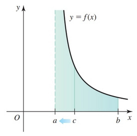
- Suppose $f$ is continuous on $(a, b]$ with $\lim_{x \to a^+} f(x) = \pm \infty$, then
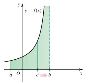
- Suppose $f$ is continuous on $[a, b)$ with $\lim_{x \to b^-} f(x) = \pm \infty$, then
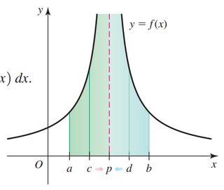
- Suppose $f$ is continuous on $[a, b]$ except at the interior point $p$ where $f$ is unbounded, then
If the limits exist then the improper integrals converge; otherwise, they diverge. If you have a solution that is composed of two limits, both limits must exist; otherwise the improper integral is divergent.
We use the same method to solve these integrals. However, We solve for the finite term and then analyze the term that is going to give us a trouble e.g. $\infty$.
$$ \begin{align} \lim_{a \to \infty} \left[-\frac{1}{x}\right]_1^a\\ = \lim_{a \to \infty} \left[-\frac{1}{a} + 1\right]_1^a\\ = 1 \end{align} $$As $a \to \infty$, $-\frac{1}{a} \to 0$, so we have $1$.
As mentioned, some will not exist:
$$ \begin{align} \lim_{a \to 0^+} \left[-\frac{1}{x}\right]_a^2\\ = \lim_{a \to 0^+} \left[-\frac{1}{2} - \overbrace{\left(-\frac{1}{a}\right)}^{\text{grows without bound}}\right]_a^2\\ = \text{DNE} \end{align} $$Given $\int_{-\infty}^{\infty} \tan^{-1} x dx$ we have:
$$ \begin{align} \lim_{a \to -\infty} [\tan^{-1}x]_a^0 + \lim_{b \to \infty} [\tan^{-1}x]_0^b\\ \lim_{a \to -\infty} [\pi/2 - \overbrace{\tan^{-1}(a)}^{\text{approaches }0}] + \lim_{b \to \infty} [\overbrace{\tan^{-1}b}^{\text{approaches }0} - \pi/2]\\ = \pi/2 + \pi/2\\ = \pi \end{align} $$Recall that if a graph is discontinuous then it is not integrable. In some cases we can determine an improper integral through careful analysis. Given:
$$ \begin{align} \int_{-1}^{1} \frac{dx}{x} \end{align} $$Note that the function is not continuous at $x = 0$ and so it is integrable only for $x \ne 0$
Sources
- Calculus: Early Transcendentals by Briggs, Cochran, Gillett
- https://www.khanacademy.org/math/integral-calculus