Derivatives
Fundamental Concepts
Differential calculus, which is primarily about derivatives, is all about instantaneous rates of change, e.g. what is the instantaneous velocity of a car right now as opposed to average velocity over a time frame. More generally, we are trying to determine the slope of a function at a given point, i.e. the slope of a line tangent to the function at a point.
The main difference between a differential and a derivative is that a differential is an infinitesimal change in a variable, while a derivative is a measure of how much the function changes for its input. The derivative measures a rate of change, while the differential measures the change itself.
Given a function such as position function $s(t)$ (where $t$ is time) we can calculate average rate of change (average velocity in this case) with the equation:
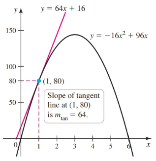
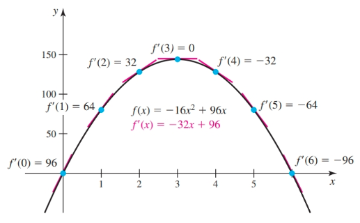
$$ \begin{align} v_{av} = \frac{s(t_1) - s(t_0)}{t_1 - t_0} \end{align} $$Given position function $s(t) = -16t^2 + 96t$ and times $t = 1$ and $t = 3$ we find the average velocity to be:
$$ \begin{align} v_{\text{av}} = \frac{288 - 144}{3 - 1}\\ = \frac{64}{2}\\ = 32 \text{ft/s} \end{align} $$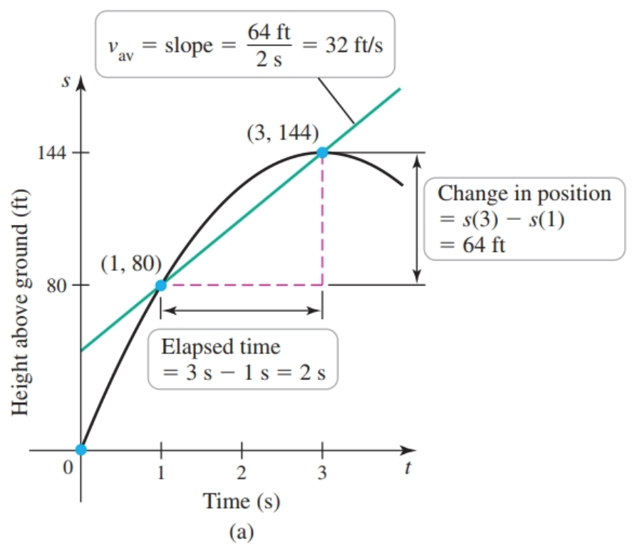
A line that joins two points on a curve, such as the one above, is called a secant line ($m_{\sec}$).
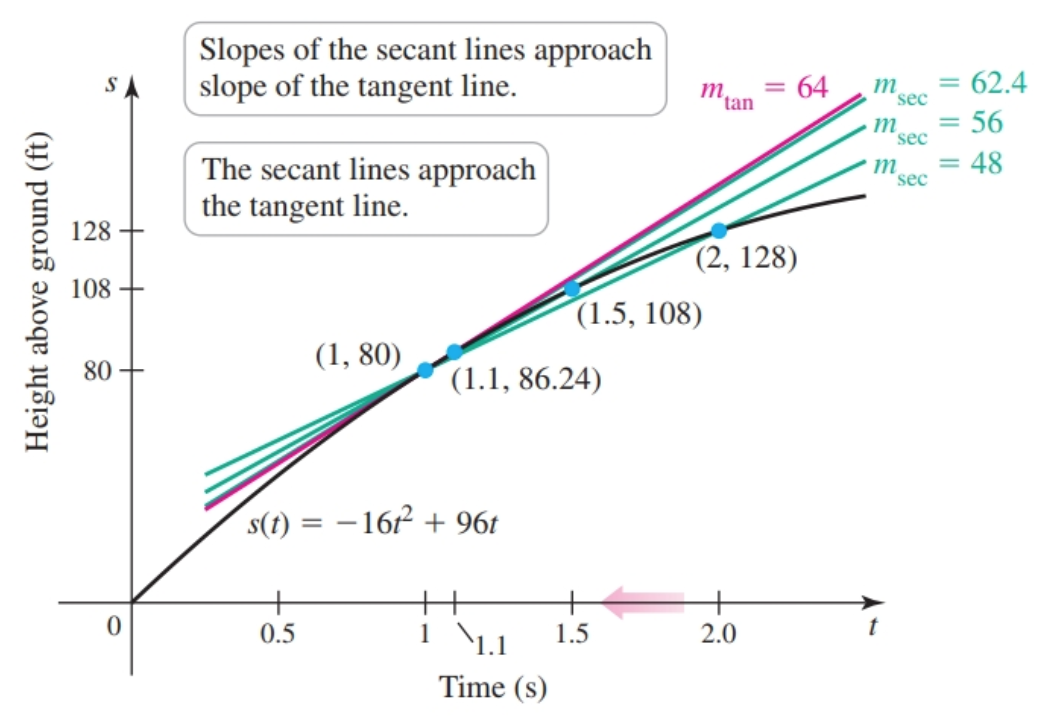
One thing to notice is that it does a pretty good job of estimating the tangent line for a point between these points, and so it can be used to estimate the slope of the tangent line (AKA instantaneous rate of change AKA derivative at this point) of the point between these two points.
As the difference between $t_1$ and $t_0$ approaches $0$ (i.e. gets smaller) the result approaches the instantaneous rate of change which is a unique number, in fact it is the limit.
$$ \begin{array}{ | c | c | c |} \hline t & s(t) & v_{\text{av}}\\ \hline 2 & 128 & 48 \\ \hline 1.5 & 108 & 56 \\ \hline 1.1 & 86.24 & 62.4 \\ \hline 1.01 & 80.638 & 63.84 \\ \hline 1.001 & 80.063984 & 63.984 \\ \hline 1.0001 & 80.00639984 & 63.9984 \\ \hline \end{array} $$The average rate of change on the interval $[1, 1.0001]$ is $63.9984$ft/s. Because this time interval is so short, it is a good approximation of the instantaneous rate of change, or limit, of $64$ft/s at $t = 1$.
This value (the limit) also happens to be the slope of a tangent line i.e. a line tangent to the curve.
We can express all of this with:
$$ \begin{align} m_{\tan} = \lim_{t \to a} \frac{s(t) - s(a)}{t - a}\\ \end{align} $$Where $a$ is the the time of interest. When $a = 1$, we have:
$$ \begin{align} m_{\tan} = \lim_{t \to 1} \frac{s(t) - s(1)}{t - 1} = 64 \end{align} $$When this limit is derived from a position function it is instantaneous velocity ($v_{\text{inst}}$).
$$ \begin{align} v_{\text{inst}} = \lim_{t \to 1} \frac{s(t) - s(1)}{t - 1} \\ = \frac{-16t^2 + 96t - 80}{t - 1}\\ = \frac{-16(t^2 - 6t + 5)}{t - 1}\\ = \frac{-16(t - 1)(t - 5)}{t - 1}\\ = -16(t - 5)\\ = 64\text{ft/s} \end{align} $$This is, in fact, the way to find the instantaneous rate of change for a specific value of $x$. Later a method will be shown to find the derivative of $f(x)$, which can be used to find the instantaneous rate of change for any value of $x$.
In simpler terms, let’s say the function $f(t)$ gives the distance in $\text{km}$ Bob has traveled at time $t$ in hours. If the derivative of $f(t)$, expressed as $f'(t)$, is equal to $100$ at $t = 2 \text{ hours}$, then we know that at $2 \text{ hours}$ Bob is traveling at a rate of $100 \text{ km}$ per hour.
$$ \begin{gather} \lim_{t \to 2} = \frac{f(t) - f(2)}{t - 2} = 100 \text{km}/\text{hr} \end{gather} $$Another way to think about this is we are trying to find the limit of the change in $y$ over the change in $x$ as the change in $x$ approaches $0$:
$$ \begin{gather} \lim_{\Delta x \to 0} \frac{\Delta y}{\Delta x} \end{gather} $$Let $f$ be a function. The derivative function, denoted by $f'$, is the function whose domain consists of those values of $x$ such that the following limit exists:
$$ \begin{gather} f'(x) = \lim_{h \to 0} \frac{f(x + h) - f(x)}{(x + h) - x}\\ = \lim_{h \to 0} \frac{f(x + h) - f(x)}{h}\\ \end{gather} $$- this is Lagrange’s notation and is pronounced “$f$ prime”
- another variation of this is $y'$ when our equation is like $y = f(x)$
There is another equivalent definition in terms of $x$ approaching $a$:
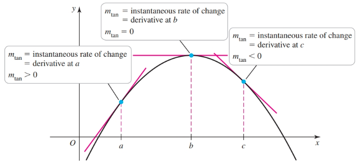
$$ \begin{gather} m_{\tan} = \lim_{x \to a} \frac{f(x) - f(a)}{x - a} \end{gather} $$Put another way, under ideal circumstances, the derivative of function $f$ is a function $f'$ that gives the slopes of lines tangent to $f$. If $x$ is our independent variable and $y$ is our dependent variable, then the derivative can be thought of as the instantaneous rate of change of $y$ with respect to $x$. Since time is often the independent variable, you will often see something like rate of change of velocity with respect to time. The process of finding a derivative is known as differentiation.
Regardless of the notation they all represent the slope at an infinitely small change in $y$ at $x$, i.e. the slope of the tangent line at $x$.
Given the function $f$, the derivative of $f$ can also be expressed as
$$ \begin{gather} \frac{d}{d x}f(x)\\ \end{gather} $$- we say “derivative with respect to $x$”
When we have an equation $y = f(x)$ we can express the derivative as
$$ \begin{gather} \frac{dy}{dx} \end{gather} $$Both of these are known as differential notation AKA Leibniz’s notation.
The following notation is found in some physics and real-world contexts is:
$$ \begin{gather} \dot f \end{gather} $$The derivative of $y = f(x)$ is expressed as:
$$ \begin{gather} \dot y \end{gather} $$These are both examples of Newton’s notation.
In any case, know that with these examples with $x$ as the independent variable and $y$ as the dependent variable, and regardless of notation, we are trying to find “the derivative of $y$ with respect to $x$.” That is we are trying to find a function of $x$ that gives the instantaneous rate of change of $y$.
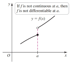
A function is said to be differentiable at $a$ if $f'(a)$ exists. More generally, a function is said to be differentiable on $S$ if it is differentaible at every point in an open set $S$. A differentiable function $f$ is one in which $f'(x)$ exists on its domain. If $f$ is not continuous at $a$, then $f$ is not differentiable at $a$.
Differentiable
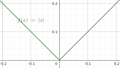
Not Differentiable for $(-\infty, \infty)$
Given the function:
$$ \begin{gather} f(x) = \left\{ \begin{array}{lr} x^2 & : x < 3\\ 6x - 9 & : x \ge 3 \end{array} \right. \end{gather} $$We see that it is continuous since:
$$ \begin{gather} \lim_{x \to 3^-} x^2 = 9\\ \lim_{x \to 3^+} 6x - 9 = 9\\ \end{gather} $$Now, we can check for differentiability:
$$ \begin{gather} \lim_{x \to 3} \frac{f(x) - f(3)}{x - 3}\\ = \frac{f(x) - 9}{x - 3} \end{gather} $$Checking from left-hand side we see that it is differentiable:
$$ \begin{gather} \lim_{x \to 3^-} \frac{x^2 - 9}{x - 3}\\ = \frac{(x + 3)(x - 3)}{x - 3}\\ = x + 3\\ = 6 \end{gather} $$Checking from the right-hand side we see that it is differentiable:
$$ \begin{gather} \lim_{x \to 3^+} \frac{6x - 9 - 9}{x - 3}\\ = \frac{6x - 18}{x - 3}\\ = \frac{6(x - 3)}{x - 3}\\ = 6 \end{gather} $$Note that the instantaneous rate of change is equal for both so this piecewise function is differentiable.
Note that differentiability implies continuity, but the converse is not true.
Slopes of Tangent Lines
Finding the slope of a tangent line
Given a value for $a$ substitute $a$ and $f(a)$ into the formula below (leave $x$ as is) to find the slope of a line tangent to $f(x)$ at $a$:
$$ \begin{gather} m_{\tan} = \lim_{x \to a} \frac{f(x) - f(a)}{x - a} \end{gather} $$Our goal is an end formula that can be solved with direct substitution such as $-16\lim_{x \to 1} (x - 5) = 64$ note that this equation is different from the derivative of $f(x)$. In particular, this formula allows us to find the slope of one tangent line.
Average rate of change and instantaneous rate of change
We can find the average rate of change, a secant line, on the interval $[a, a + h]$ with
$$ \begin{gather} m_{\sec} = \frac{f(a + h) - f(a)}{a + h - a} \\ = \frac{f(a + h) - f(a)}{h} \\ \end{gather} $$- Substitute $a$ and $h$ into the formula
We may find the instaneous rate of change (the slope of the tangent line) with the following limit:
$$ \begin{gather} m_{\tan} = \lim_{h \to 0} \frac{f(a + h) - f(a)}{h} \end{gather} $$- Given a value for $a$ substitute $a$ and $f(a)$ into the formula.
- Once $h$ is factored out of the denominator, substitute in $0$ for $h$
Our end goal is a formula that can be solved by direct substitution of $h$ such as:
$$ \begin{gather} \lim_{h \to 0} (h^2 + 3h + 7) = 7 \end{gather} $$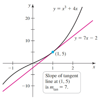
Equation of a Tangent Line
If we are given point $P(a, b)$ and have found the slope the tangent line $m$ then it is trivial to find the equation for the tangent line:
$$ \begin{gather} y - a = m(x - b)\\ y = m(x - b) + a \end{gather} $$More concretely, given $P(3, -4)$ and $m_{tan} = -2$, we have:
$$ \begin{gather} y = -2x + 2 \end{gather} $$Calculating the Derivative Numerically
Version 3
We can find the derivative by simplifying the following limit:
$$ \begin{gather} f'(x) = \lim_{h \to 0} \frac{f(x + h) - f(x)}{h} \end{gather} $$Given $f(x) = -16x^2 + 96x$ the end goal is a limit that can be solved with direct substitution:
$$ \begin{gather} f'(x) = \lim_{h \to 0} \frac{[-16(x + h)^2 + 96(x + h)] - [-16x^2 + 96x]}{x + h - x}\\ = \frac{-16(x^2 + 2xh + h^2) + 96x + 96h + 16x^2 - 96x}{h}\\ = \frac{-16x^2 - 32xh - 16h^2 + 96h + 16x^2}{h}\\ = \frac{-32xh - 16h^2 + 96h}{h}\\ = -32x - 16h + 96 \end{gather} $$Now, we solve with direct substitution for $h$:
$$ \begin{gather} f'(x) = \lim_{h \to 0} -32x - 16h + 96 = -32x + 96 \end{gather} $$So, for any $x$, $f'(x)$ gives the instantaneous rate of change at $f(x)$.
Derivative Notation
- a derivative with respect to $x$ is generally expressed as $f'(x)$ (read as “$f$ prime”), $y'(x), D_x (f(x))$ Or, deriving from $\Delta$ notation, $\frac{df}{dx}, \frac{dy}{dx}$ (read as “the derivative of $y$ with respect to $x$” or “$dy$ $dx$”), $\frac{d}{dx}(f(x))$.
- When a derivative is evalutated at $a$ we have $f'(a), y'(a), \frac{df}{dx}|_{x = a}, \frac{dy}{dx}|_{x = a}$
$\Delta$ Notation
Using $\Delta x$ and $\Delta y$ we can express a secant line as:
$$ \begin{gather} m_{\sec} = \frac{f(x + \Delta x) - f(x)}{\Delta x} = \frac{\Delta y}{\Delta x} \end{gather} $$If we turn this into a limit where $\Delta \to 0$ we have the derivative function:
$$ \begin{gather} f'(x) = \lim_{\Delta x \to 0} \frac{f(x + \Delta x) - f(x)}{\Delta x} \end{gather} $$If we take the limit as $\Delta \to x$ we have the slope of a tangent line at $(x, f(x))$
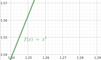
$$ \begin{gather} m_{\tan} = \lim_{\Delta \to x} \frac{\Delta y}{\Delta x} \end{gather} $$Given the function $f(x) = x^2$ we can find the derivative at a specific point with the formal definition. Here we want to find the slope at the point $x = 3$.
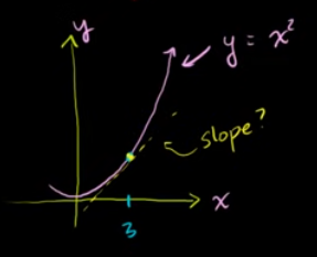
Let’s find the slope between it and another arbitrary point $(3 + \Delta x)$ giving us a secant line.
For $x = 3$ we have $(3, 9)$ for $x = 3 + \Delta x$ we have $(3 + \Delta x, (3 + \Delta x)^2).
Solving for the following gives us a formula which we can use to find the instantaneous slope (the derivative) relative to $3$:
$$ \begin{gather} \frac{\Delta y}{\Delta x} = \frac{(3 + \Delta x)^2 - 9}{3 + \Delta x - 3}\\ = \frac{9 + 6 \Delta x + \Delta x^2 - 9}{3 + \Delta x - 3}\\ = \frac{6 \Delta x + \Delta x^2}{\Delta x}\\ = 6 + \Delta x \end{gather} $$If we want to find the slope at $x = 3$ we find the following limit:
$$ \begin{gather} \lim_{\Delta x \to 0} 6 + \Delta x = 6 = f'(3) \end{gather} $$Rules of Differentiation
Instead of using the limit definition to find a derivative, we can compute derivatives much faster by using the rules of differentiation.
- used to calculate derivatives without using derivative formulas
- beware constants that do not appear to be constants e.g. $\ln 5$, $e^7$, etc.
Basics of Differentiation
Observe that an equation such as $y = 7x^2 + 4x + 7$ can be thought of as the sum of multiple functions i.e. $y = g(x) + h(x) + i(x)$. And, we can treat the whole right side as a single function $f(x)$ as in $y = f(x)$.
Further we can treat some functions as compositions:
$$ \begin{gather} f(x) = \sin(x^2) = g(h(b)), g(a) = \sin(a), h(b) = b^2 \end{gather} $$Given an equation:
$$ \begin{gather} y = f(x) \end{gather} $$We differentiate with respect to $x$ when we do the following:
$$ \begin{gather} \frac{dy}{dx} = \frac{d}{dx}[f(x)] \end{gather} $$What should be understood is that $\frac{dy}{dx}$ is a variable (standing in for our derivative), and the $\frac{d}{dx}$ represents a function whose result is the value of left-hand side (the derivative).
Given an equation with respect to $y$ that is a sum of terms:
$$ \begin{gather} y = f(x) + g(x) \end{gather} $$We differentiate with:
$$ \begin{gather} \frac{dy}{dx} = \frac{d}{dx}[f(x)] + \frac{d}{dx}[g(x)] \end{gather} $$If we replace the $+$ with a $-$ we have something similar:
$$ \begin{gather} \frac{dy}{dx} = \frac{d}{dx}[f(x)] - \frac{d}{dx}[g(x)] \end{gather} $$Differentiation with Constants
Coefficients can be brought outside and back in:
$$ \begin{gather} y = 3x^2\\ y = 3f(x)\\ \end{gather} $$$$ \begin{gather} y' = 3 \frac{d}{dx}[f(x)]\\ \end{gather} $$More formally, we have:
$$ \begin{gather} \frac{d}{dx}[c] = 0, c \in \mathbb{R}\\ \frac{d}{dx}(cx) = (0)(x) + (c)(1) = c, c \in \mathbb{R}\\ \end{gather} $$(See the product rule)
Examples
$$ \begin{gather} \frac{d}{dx}(7) = 0\\ \frac{d}{dx}(7x) = 7 \end{gather} $$The Product Rule
If instead we have:
$$ \begin{gather} y = f(x) \cdot g(x) \end{gather} $$We use the product rule to combine two terms:
$$ \begin{gather} y' = f'(x) \cdot g(x) + g'(x) \cdot f(x) \end{gather} $$The Quotient Rule
If instead we have:
$$ \begin{gather} y = \frac{f(x)}{g(x)} \end{gather} $$We use the quotient rule to combine two terms:
$$ \begin{gather} y' = \frac{f'(x) \cdot g(x) - g'(x) f(x)}{g^2(x)} \end{gather} $$One strategy to use for rational functions such as:
$$ \begin{gather} y = \frac{5 - 3x}{x^2 + 3x} \end{gather} $$is to perform substitutions that simplify the equation:
$$ \begin{gather} y = \frac{5 - 3x}{x^2 + 3x} = \frac{u(x)}{v(x)} \end{gather} $$}
Developing an Intuition for Derivatives
Notice the relationship between a constant function and its derivative:
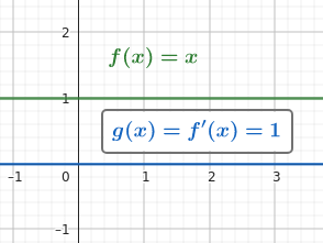
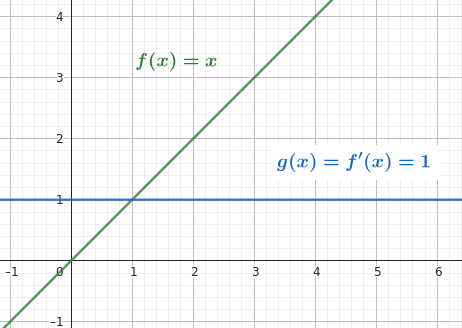
Notice the relationship between a linear equation and its derivative:
Notice the relationship between a polynomial and its derivative:

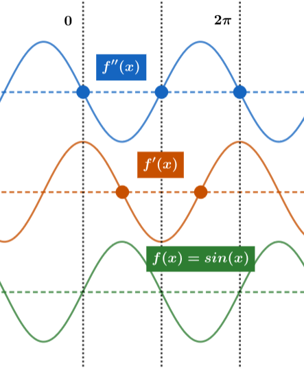
Notice the relationship between $\sin x$ and its derivative:
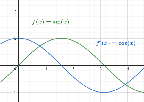
Notice the relationship between $\cos x$ and its derivative:
![$\frac{d}{dx}\left[\cos(x) \right] = -\sin(x)](./img/derivatives-39.png)
Differentiation of Logarithms and Powers
The power rule is expressed as:
$$ \begin{gather} \frac{d}{dx} [x^n] = n(x)^{n-1}\\ \end{gather} $$$$ \begin{gather} \frac{d}{dx} [\sqrt{x}] = \frac{1}{2\sqrt{x}}\\ \frac{d}{dx} [e^{x}] = e^{x}\\ \frac{d}{dx} [e^{g(x)}] = e^{g(x)} \cdot g'(x)\\ \frac{d}{dx} [\ln x] = \frac{d}{dx} [\ln |x|] = \frac{1}{x}, x \ne 0\\ \frac{d}{dx} [\ln x] = \frac{d}{dx} [\ln g(x)] = \frac{1}{g(x)} \cdot g'(x), x \ne 0\\ \frac{d}{dx} [\ln k] = 0, \text{when }k \text{ is a constant!}\\ \frac{d}{dx} [b^x] = b^x \ln b\\ \frac{d}{dx} [\log_b x] = \frac{1}{x \ln b}\\ \frac{d}{dx} [\ln(f(x))] = \frac{f'(x)}{f(x)}\\ \frac{d}{dx} [x^x] = x^x(\ln(x) + 1)\\ \end{gather} $$Examples
$$ \begin{gather} \frac{d}{dx}(x) = (1)x^{1 - 1} = 1\\ \frac{d}{dx}(x^5) = 5x^4\\ \frac{d}{dx}(x^{-5}) = -5x^{-6} = \frac{d}{dx}(1)/\frac{d}{dx}(n^5)\\ \frac{d}{dx}(x^{\frac{1}{2}}) = \frac{1}{2}x^{-\frac{1}{2}}\\ \frac{d}{dx}(n^5) = 5n^4, \frac{d}{dx}(n^{-5}) = -5n^{-6} = \frac{d}{dx}(1)/\frac{d}{dx}(n^5)\\ \end{gather} $$Differentiating Trigonometric Functions
$$ \begin{gather} \frac{d}{dx}(\sin x) = \cos x\\ \frac{d}{dx}(\cos x) = -\sin x\\ \frac{d}{dx}(\tan x) = \frac{d}{dx}\left[\frac{\sin x}{\cos x}\right] = \dots = \sec^2 x\\ \frac{d}{dx}(\cot x) = \frac{d}{dx}\left[\frac{\cos x}{\sin x}\right] = \dots = -\csc^2 x\\ \frac{d}{dx}(\sec x) = \frac{d}{dx} \left[\frac{1}{\cos x}\right] = \dots = \sec x \tan x\\ \frac{d}{dx}(\csc x) = \frac{d}{dx} \left[\frac{1}{\sin x}\right] = \dots = -\csc x \cot x \end{gather} $$Special cases for trigonometric functions
When there is a constant $a$ on $x$, it remains on every $x$ in the derivative, but is also brought out front of the resulting expression e.g.:
$$ \begin{gather} \frac{d}{dx}(\sin ax) = a\cos ax\\ \end{gather} $$When there is a constant $k$ on the trigonometric function, it remains on the derivative e.g.:
$$ \begin{gather} \frac{d}{dx}(k\sin x) = k\cos x\\ \end{gather} $$Differentiating Inverse Trig Functions
$$ \begin{gather} \frac{d}{dx}[\sin^{-1}(x)] = \frac{1}{\sqrt{1 - x^2}}\\ \frac{d}{dx}[\cos^{-1}(x)] = -\frac{1}{\sqrt{1 - x^2}}\\ \frac{d}{dx}[\tan^{-1}(x)] = \frac{1}{1 + x^2}\\ \frac{d}{dx}[\cot^{-1}(x)] = -\frac{1}{x^2 + 1}\\ \frac{d}{dx}[\sec^{-1}(x)] = \frac{1}{|x| \sqrt{x^2 - 1}}\\ \frac{d}{dx}[\csc^{-1}(x)] = -\frac{1}{|x| \sqrt{x^2 - 1}}\\ \end{gather} $$- Note that setting $a = 1$ in the above equations offers simpler versions of these identities
Consider $y = \sin^{-1}(x)$. We can rewrite this as $\sin(y) = x$. And, now we can use implicit differentiation to find the derivative of $\sin^{-1}(x)$:
$$ \begin{gather} \frac{d}{dx}[\sin(y)] = \frac{d}{dx}(x)\\ \frac{dy}{dx} \cdot \cos(y) = 1\\ \frac{dy}{dx} = \frac{1}{\cos(y)} \end{gather} $$We still need the RHS in terms of $x$. We already have $x = \sin(y)$ and we know from trigonometry $\cos(y) = \sqrt{1 - \sin^2 y}$ so:
$$ \begin{gather} \frac{dy}{dx} = \frac{1}{\sqrt{1 - \sin^2y}}\\ = \frac{1}{\sqrt{1 - x^2}} \end{gather} $$A similar method can be used to find the derivative of other trigonometric functions.
The Chain Rule
Expressions like $(x + 5)^{100}$ are hard to differentiate – the chain rule makes differentiating such expressions easier. The chain rule tells us how to find the derivative of a composite function. The trick is to think of this as two functions:
$$ \begin{gather} g(u) = u^{100} u = h(x) = x + 5 \end{gather} $$If we have:
$$ \begin{gather} y = f(x) \end{gather} $$And, $f(x)$ can be treated as a composition of functions:
$$ \begin{gather} y = f(g(x)) \end{gather} $$We can set $u$ to $g(x)$, i.e. $u = g(x)$, and rewrite the expression:
$$ \begin{gather} y = f(u) \end{gather} $$Now, we use the chain rule:
$$ \begin{gather} y' = f'(u) \cdot u' \end{gather} $$And, finally substitute $g(x)$ back in:
$$ \begin{gather} y' = f'(g(x)) \cdot u'\\ = f'(g(x)) \cdot g'(x) \end{gather} $$Equivalently, the chain rule is expressed this way:
$$ \begin{gather} \frac{dy}{dx} = \frac{dy}{du} \cdot \frac{du}{dx} \end{gather} $$Regard $du/dx$ as the rate of change of $u$ with respect to $x$, $dy/du$ as the rate of change of $y$ with respect to $u$, and $dy/dx$ as the rate of change of $y$ with respect to $x$. If $u$ changes twice as fast as $x$ and $y$ changes three times as fast as $u$, then it seems reasonable that $y$ changes six times as fast as $x$, and so we expect the above to be true.
Strategies
$$ \begin{gather} \frac{d}{dx}[(x^2 + 3x)^3] = \frac{d}{du}(u^3) \cdot \frac{d}{dx}(x^2 + 3x) = 3(x^2 + 3x)^2 \cdot (2x + 3)\\ \frac{d}{dx}[e^{4x^3 + 1}] = \frac{d}{du}(e^u) \cdot \frac{d}{dx}(4x^3 + 1) = e^{4x^3 + 1} \cdot 8x^2\\ \frac{d}{dx}[\sin(3x^2 + 4)] = \frac{d}{du}(\sin(u)) \cdot \frac{d}{dx}(3x^2 + 4) = \cos(3x^2 + 4) \cdot 6x\\ \frac{d}{dx}[e^{g(x)}] = g'(x) \cdot e^{g(x)} \frac{d}{dx}[sin^2 x] = \frac{d}{dx} [ (\sin x)^2] = 2 \sin x \cos x \end{gather} $$Higher-Order Derivatives
We can take the derivative of the derivative of $f$. The result is the second derivative of $f$, denoted $f''$ (read as “$f$ double prime”). Derivatives of order $n \geq 2$ are called higher-order derivatives
Consider again the example of $f(t)$ which gives distance in kilometers at time in hours $t$. The first derivative gives the instantaneous velocity. If we want to know the instantaneous rate of change of velocity – i.e. acceleration – we take the derivative of the derivative (the second derivative).
Second derivative:
$$ \begin{gather} f''(x) = \frac{d}{dx}(f'(x)) \end{gather} $$For fourth derivatives and beyond:
$$ \begin{gather} f^{(n)} (x) = \frac{d}{dx}(f^{(n - 1)}(x)) \end{gather} $$Parentheses are used to distinguish $f^{(n)}$ from $f^n$.
Other common notations for the second derivative of $y = f(x)$ include $\frac{d^2f}{dx^2}$ and $\frac{d^2y}{dx^2}$. The last one stems from $\left(\frac{d}{dx}(\frac{df}{dx})\right)$ and is read “$d$ $2$ $f$ $d$ $x$ squared.” And, the other stems from $\frac{d}{dx}[\frac{d}{dx}[y]]$.
In general, the $n$th derivative of an $n$th degree polynomial is a constant, which implies that derivatives of order $k > n$ are $0$.
Implicit Differentation Example
We have that $\dfrac{dy}{dx} = e^{5y}$, and we need to find $\dfrac{d^2y}{dx^2}$ in terms of $x$ and $y$.
$$ \begin{gather} \dfrac{d^2y}{dx^2} = 5e^{5y} \cdot \dfrac{dy}{dx}\\ = 5e^{10y} \end{gather} $$Another Example
We are given the following:
$$ \begin{gather} y = \sqrt{x}\\ \frac{dx}{dt} = 12\\ \end{gather} $$What is $\frac{dy}{dt}$ when $x = 9$?
Notice that we differentiating with respect to $t$.
Think of it like this – both $x$ and $y$ are functions of $t$, i.e. $x = f(t)$ and $y = \sqrt{f(t)}$. We can apply the chain rule. So, we have:
$$ \begin{gather} \frac{dy}{dt} = \frac{dy}{dx} \cdot \frac{dx}{dt}\\ = \frac{1}{2}x^{-\frac{1}{2}} \cdot 12\\ = 2 \end{gather} $$Another example
Given:
$$ \begin{gather} \sin(x) + \cos(y) = \sqrt{2} \end{gather} $$Find $\frac{dy}{dt}$.
Think of $x$ and $y$ as $x(t)$ and $y(t)$, respectively. So, we have:
$$ \begin{gather} \sin(x(t)) + \cos(y(t)) = \sqrt{2} \end{gather} $$We are differentiating with respect to $t$, so:
$$ \begin{gather} \frac{d}{dt}[\sin(x(t))] + \frac{d}{dt}[\cos(y(t))] = \frac{d}{dt}[\sqrt{2}]\\ \end{gather} $$We use the chain rule:
$$ \begin{gather} \frac{dx}{dt} \cdot \cos(x) + \frac{dy}{dt} \cdot -\sin(y) = 0\\ \frac{dy}{dt} \cdot -\sin(y) = - \frac{dx}{dt} \cdot \cos(x)\\ \frac{dy}{dt} = \frac{\frac{dx}{dt}\cos(x)}{-\sin(y)} \end{gather} $$This relevant to related rate problems. In a real-world context, this can be useful for a variety of problems such as having $y$ of one chemical and $f(x)$ (a function of $x$ such $\sqrt{x}$) of another chemical at time $t$ and we want to find the change in one variable with respect to $t$.
Going from Limits to Derivatives
We are presented with the following limit:
$$ \begin{gather} \lim_{h \to 0} \frac{f(x + h) - f(x)}{h} \end{gather} $$The derivative is simply $f'(x)$. If $x$ is defined we find $f'(x)$.
Strategies for Differentiation
- ways to approach solutions
- use the natural logarithm
- substitute trigonometric identities e.g $\frac{sin x}{x} = 1$
- given a limit where $\lim_{x \to 3}$ substitute an expression such as $(x - 3)$ for $t$ for a new limit where $\lim_{t \to 0}$
- use a table or graph to determine that the limit exists and find its value
Implicit Differentiation
Variation 1
Consider the following equation for a circle:
$$ \begin{gather} x^2 + y^2 = 1 \end{gather} $$In such an equation, the values of $x$ and $y$ are explicit. In other words, the equation isn’t of a form such as:
$$ \begin{gather} y = \dots \end{gather} $$In this case we can use a special method for finding the derivative.
$$ \begin{gather} \frac{d}{dx}[ x^2 + y^2] = \frac{d}{dx}[1]\\ \frac{d}{dx}[x^2] + \frac{d}{dx}[y^2] = 0\\ 2x + \frac{d}{dx}[y^2] = 0 \end{gather} $$This is where the chain rule comes in. $y^2$ is the outer function, and $y$ is the inner function. We need the change in $y$ with respect to $y^2$ and we also need the change in $y$ with respect to $x$. So, we have:
$$ \begin{gather} 2x + \frac{d(y^2)}{dy} \cdot \frac{dy}{dx} = 0 \end{gather} $$It might be easier to think about $\frac{d}{dx}[y^2]$ in this way:
$$ \begin{gather} \frac{d}{dx}[y^2] = \frac{d}{dx}[(y(x))^2] \end{gather} $$Continuing with the problem, we have:
$$ \begin{gather} 2x + \frac{d(y^2)}{dy} \cdot \frac{dy}{dx} = 0\\ 2x + 2y \cdot \frac{dy}{dx} = 0\\ 2y \cdot \frac{dy}{dx} = - 2x\\ \frac{dy}{dx} = \frac{-2x}{2y}\\ \frac{dy}{dx} = \frac{-x}{y} \end{gather} $$Variation 2
There may be cases where the relationship between terms is explicitly defined e.g $y$ in terms of $x$:
$$ \begin{gather} y = 2x + 3 \end{gather} $$In other problems the relationship between variables is implicit:
$$ \begin{gather} 2y^5 = 4x^3 + 4 \end{gather} $$We can see this again in terms of functions:
$$ \begin{gather} y(x) = \underbrace{f(x) + g(x)}_{\text{combine this into one function}}\\ y(x) = f(x) \end{gather} $$When the relationships are implicit, we can leverage the chain rule and differentiate with respect to $x$ this way:
$$ \begin{gather} \frac{dy}{dx} \frac{d}{dx}(y(x)) = \frac{d}{dx}(f(x)) \end{gather} $$Given $2y^5 = 4x^3 + 4$ and differentiating with respect to $x$, we have:
$$ \begin{gather} \frac{dy}{dx} \frac{d}{dx}(2y^5) = \frac{d}{dx}(4x^3 + 4)\\ \frac{dy}{dx} 10y^4 = 12x^2\\ \frac{dy}{dx} = \frac{12x^2}{10y^4} \end{gather} $$- Note that every instance of the dependent variable becomes the product of the derivative in terms of the independent variable and the derivative of itself while the independent variable becomes the derivative in terms of itself, for example:
Variation 3
It may be the case that the independent variable is not explicitly defined. Instead, all non-constant terms in the equation relate to eachother and are implicitly tied to an unexpressed independent variable. This is often the case with equations involving time. Our independent variable is $t$, where is it:
$$ \begin{gather} a^2 = 2b^5 + 4c^3 \end{gather} $$If the independent variable is $t$ we might remind ourselves by writing:
$$ \begin{gather} a(t)^2 = 2b(t)^5 + 4c(t)^3 \end{gather} $$But, this is not necessary. When we differentiate with respect to $t$ we get:
$$ \begin{gather} 2a \frac{da}{dt} = 10 b^4 \frac{db}{dt} + 12c^2 \frac{dc}{dt} \end{gather} $$If $a$ relates to meters $t$ relates to seconds, and we solve for $\frac{da}{dt}$ we find some rate of change (it’s a derivative) in terms of meters per second. If $a$ relates instead to meters$^2$ then we would be solving in terms of meters-squared per second.
Even though the equation does not allow explicit manipulation of the independent variable we can insert different values for our dependent variables to solve for different results. More simply, if time is our independent variable then we may solve for equations at $5$ seconds, $10$ seconds, etc. we need only insert the values of the dependent variables at the respective time.
- basically, when differentiating with respect to $x$, $d/dx(y) = d/dx(y) \cdot dy/dx$
where $c$ is some constant:
$$ \begin{gather} x^2 + y^2 = c\\ \frac{d}{dx}(x^2) + \frac{d}{dx}(y(x))^2 = \frac{d}{dx}(c)\\ 2x + 2y \frac{dy}{dx} = 0\\ 2y \frac{dy}{dx} = -2x\\ \frac{dy}{dx} = -\frac{2x}{2y}\\ \frac{dy}{dx} = -\frac{x}{y} \end{gather} $$Given $y$ replace with $y(x)$ whose derivative is $\frac{dy}{dx}$ Given $y^n$ replace with $(y(x))^n$ whose derivative is $(ny^{n - 1}) \left(\frac{dy}{dx}\right)$ (it is a composition) e.g. $\frac{d}{dx}(4y^3) = 12y^2 \cdot \frac{dy}{dx}$.
It is a composition of $y$ and $\frac{dy}{dx}$ Substitute $y$ for $\frac{dy}{dx}$, $cy^n$ for $cny^{n-1} \frac{dy}{dx}$
Derivatives of Inverse Functions
Given $f(x)$ and $g(x) = f^{-1}(x)$, we find that:
$$ \begin{gather} \frac{d}{dx}[g(f(x))] = \frac{d}{dx}(x)\\ g'(f(x)) \cdot f'(x) = 1\\ f'(x) = \frac{1}{g'(f(x))} \end{gather} $$Given $f(x) = e^x$ we have $f^{-1}(x) = ln x$ and $g'(x) = \frac{1}{x}$:
$$ \begin{gather} \frac{d}{dx}[e^x] = \frac{1}{\frac{1}{x}} = e^x \end{gather} $$Interpreting Graphs
Is the object speeding up, slowing down, or neither for the following points?
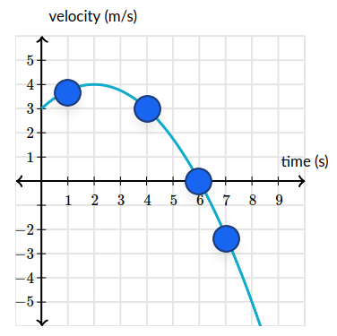
Note that speed is the magnitude of velocity (take the absolute value of velocity).
We have the following:
- Speeding up – it is going towards the maximum
- Slowing down – it is going towards $0$
- Neither – the velocity is at $0$
- Speeding up – the velocity is increasing towards the minimum
Is the object moving forward, backward or neither for the points given?
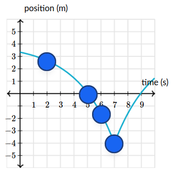
We take movement in the direction of negative numbers to be backward and vice versa for movement in the direction of positive numbers.
- Backward
- Backward
- Backward
- Neither
For each point on the graph, is the object moving forward, backward, or neither?
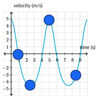
- Neither – it is moving at a velocity of $0$ which has no direction
- Backward – velocity is $\approx -4.5 \text{m}/{s}$
- Forward – velocity is $\approx 5 \text{m}/{s}$
- Backward – velocity is $\approx -3 \text{m}/{s}$
For each point on the graph, is the object speeding up, slowing down, or neither?
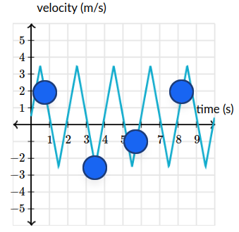
- Slowing down – retreating from the maximum
- Neither – velocity is steady
- Slowing down – retreating from the minimum
- Speeding up – moving toward the maximum
Determining Distance Traveled
Given the following position equation where $t$ is time in seconds:
$$ \begin{gather} x(t) = \frac{2}{3}t^3 - 6t^2 + 10t, \text{ for } t \ge 0 \end{gather} $$What is the total distance traveled by the particle for $0 \le t \le 6$?
We know that when velocity is zero there is a change in direction. For $v(t)$ (which is $x'(t)$) we have:
$$ \begin{gather} v(t) = 2t^2 - 12t + 10\\ 0 = 2t^2 - 12t + 10\\ = t^2 - 6t + 5\\ = (t - 5)(t - 1)\\ t = 1 \text{ or } t = 5 \end{gather} $$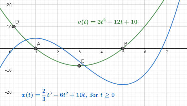
D. initial velocity of $10$ A. velocity of $0$ C. max velocity in negative/backwards direction B. velocity of $0$
We plug these times in to find the position at those times and the start and end times:
$$ \begin{gather} x(0) = 0\\ x(1) = 4\frac{2}{3}\\ x(5) = -16\frac{2}{3}\\ x(6) = -12 \end{gather} $$So, for total distance, we have:
$$ \begin{gather} |4\frac{2}{3} - 0| + |-16\frac{2}{3} - 4\frac{2}{3}| + |-12 - -16\frac{2}{3}| =\\ 4\frac{2}{3} + 21\frac{1}{3} + 4\frac{2}{3} = 30\frac{2}{3} \end{gather} $$Increasing and Decreasing Functions
We say that function $f$ is increasing on $I$ if $f(x_2) \ge f(x_1)$ whenever $x_1$ and $x_2$ are in $I$ and $x_2 \gt x_1$; if $f(x_2) \gt f(x_1)$ then $f$ is strictly increasing. We say that $f$ is decreasing on $I$ if $f(x_2) \le f(x_1)$ whenever $x_1$ and $x_2$ are in $I$ and $x_2 \gt x_1$; if $f(x_2) \lt f(x_1)$ then $f$ is strictly decreasing.
A function is called monotonic if it is either increasing or decreasing. We can make a further distinction by defining nondecreasing $(f(x_2) \geq f(x_1)$ whenever $x_2 > x_1$) and nonincreasing $(f(x_2) \leq f(x_1)$ whenever $x_2 \gt x_1)$.
Use $f'(x)$ to determine where intervals increase/decrease precisely.
Suppose $f$ is continuous on an interval $I$ and differentiable at all interior points of $I$.
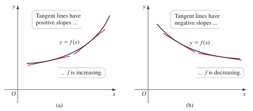
- If $f′(x) > 0$ at all interior points of $I$, then $f$ is increasing on $I$ (positive slopes for $f(x)$).
- If $f′(x) < 0$ at all interior points of $I$, then $f$ is decreasing on $I$ (negative slopes for $f(x)$).
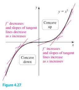
The converse of this may not be true i.e. if a function is increasing on $I$ then $f'(x) > 0$… According to the definition, $f(x) = x^3$ is increasing on $(-\infty, \infty)$ but it is not true that $f′(x) > 0$ on $(-\infty, \infty)$ (because $f′(0) = 0)$.
We can use graphs to make determinations about local and absolute maxima.
The first derivative test allows us to identify local maxima and minima.
Suppose that $f$ is continuous on an interval that contains a critical point $c$ and assume $f$ is differentiable on an interval containing $c$, except perhaps at $c$ itself.
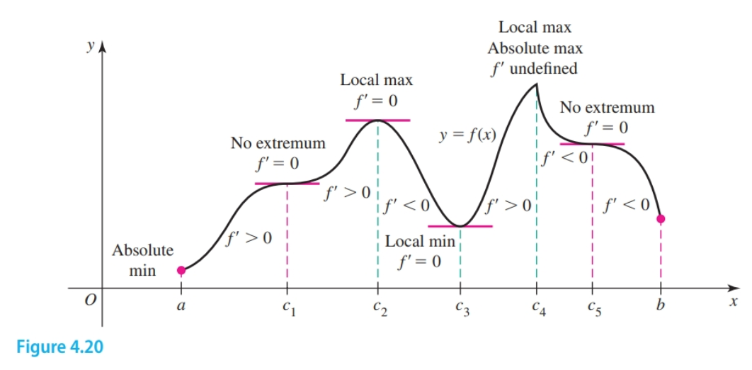
- If $f'$ changes sign from $+$ to $-$ as $x$ increases through $c$, then $f$ has a local maximum at $c$.
- If $f'$ changes sign from $-$ to $+$ as $x$ increases through $c$, then $f$ has a local minimum at $c$.
- If $f'$ has the same signs on both sides near $c$, then $f$ has no local extreme value at $c$.
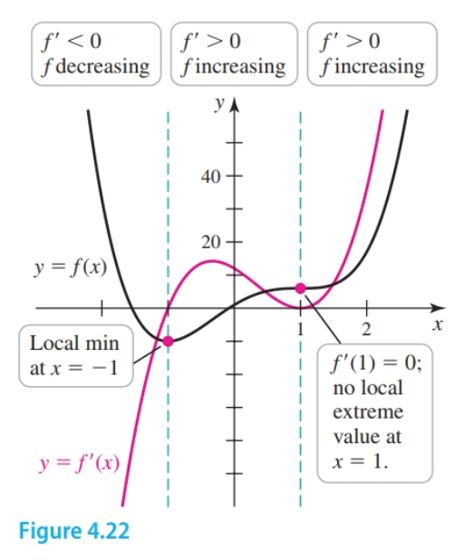
Consider the function
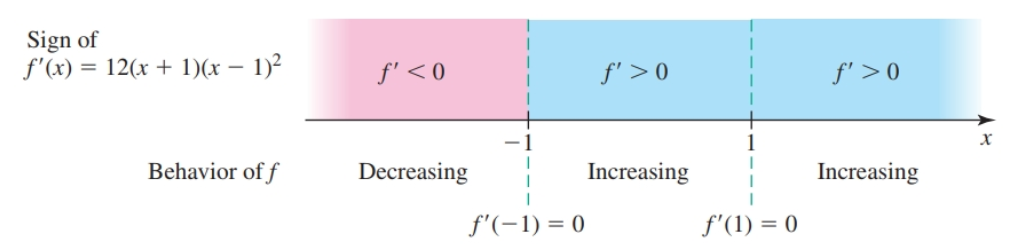
$$ \begin{gather} f(x) = 3x^4 - 4x^3 - 6x^2 + 12x + 1 \end{gather} $$With derivative:
$$ \begin{gather} f'(x) = 12(x + 1)(x - 1)^2 \end{gather} $$Solving $f'(x) = 0$ gives the critical points $x = -1$ and $x = 1$.
We test values and/or analyze the functions for the given interval, finding that there is a sign change going from the interval $(-\infty, -1)$ to $(-1, 1)$ so there is a local minimum at $x = -1$; and there is no sign change going from the interval $(-1, 1)$ to $(1, \infty)$. We can summarize the behavior of $f(x)$ with a sign graph:
Maxima and Minima
Global Maxima and Minima
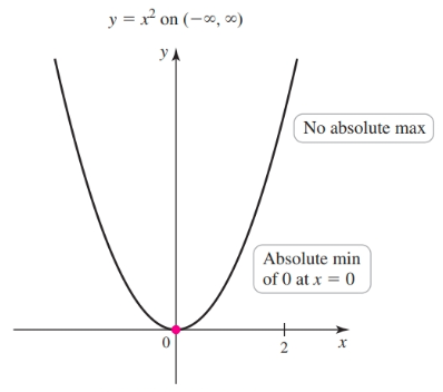
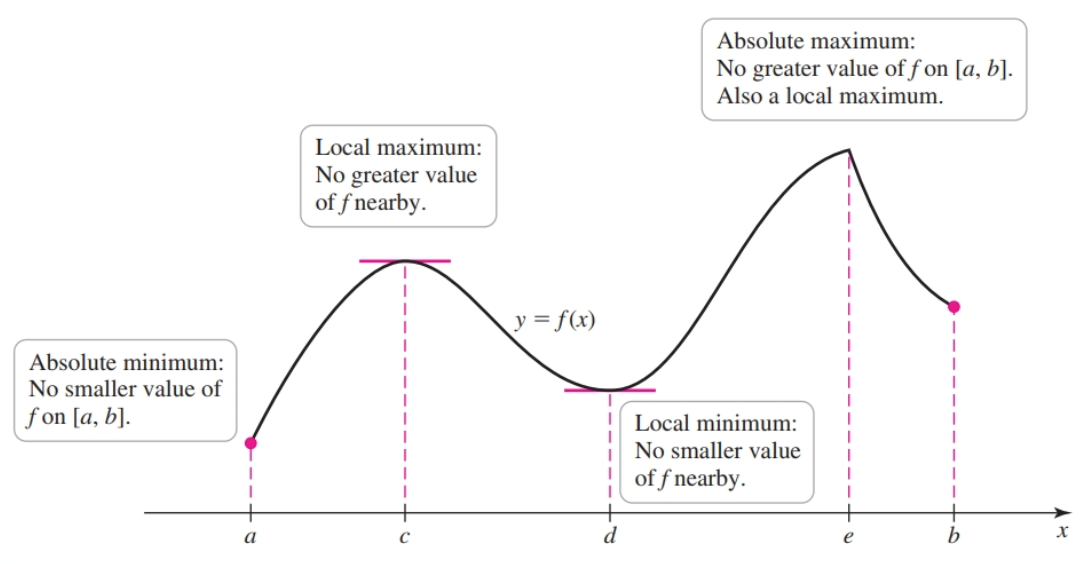
Let $f$ be defined on a set $D$ containing $c$. If $f(c) \geq f(x)$ for every $x$ in $D$, then $f(c)$ is an absolute maximum value AKA global maximum of $f$ on $D$. If $f(c) \leq f(x)$ for every $x$ in $D$, then $f(c)$ is an absolute minimum value AKA global minimum of $f$ on $D$. An absolute extreme value (extremum and extrema) is either an absolute maximum or an absolute minimum value.
The extreme value theorem says that a function that is continuous on a closed interval $[a, b]$ has an absolute maximum value and an absolute minimum value on that interval.
Other possibilities:
- there is no absolute minimum or absolute maximum.
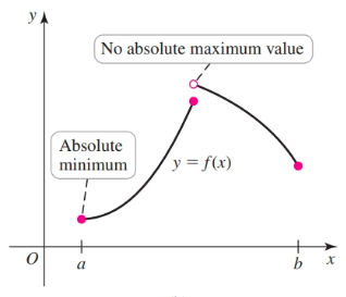
- the absolute maximum/minimum occurs in more than one place.
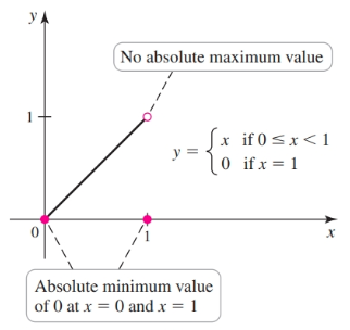
- the absolute minimum/maximum are the same value.
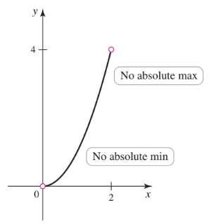
A more practical example – of a non-closed interval over a function – is a continuous function over $[0, \infty)$.
Local Maxima and Minima
Suppose $c$ is an interior point of some open interval $I = (c - h, c + h), h \gt 0$ on which $f$ is defined. If $f(c) \geq f(x)$ for all $x$ in $I$, then $f(c)$ is a local maximum value AKA relative maximum of $f$. If $f(c) \leq f(x)$ for all $x$ in $I$, then $f(c)$ is a local minimum AKA relative minimum value of $f$. One convention followed is that local maxima/minima can only be on interior points of the interval of interest i.e. they occur on open intervals.
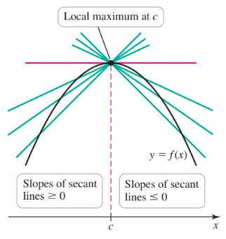
If $f$ has a local maximum or minimum value at $c$ and $f'(c)$ exists, then $f'(c) = 0$
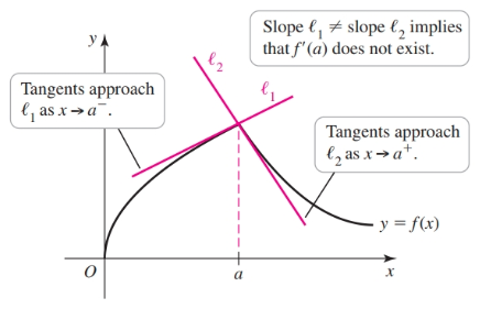
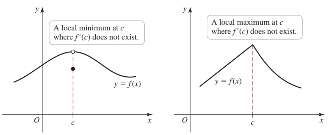
Local extrema can also occur at points $c$ where $f(c)$ does not exist. The figure below shows two such cases, one in which $c$ is a point of discontinuity and one in which $f$ has a corner point at $c$.
An interior point $c$ of the domain of $f$ at which $f'(c) = 0$ or $f'(c)$ fails to exist is called a critical point of $f$.
A critical point $a$ is a maximum if $f'(c)$ switches signs from positive to negative as we cross $c = a$. A critical point $a$ is a minimum if $f'(c)$ switches signs from negative to positive as we cross $c = a$.
A local maximum (or minimum) at $c$ necessarily implies a critical point at $c$, but a critical point at $c$ does not imply a local maximum (or minimum) there.
It is possible that $f′(c) = 0$ at a point without a local maximum or local minimum value occurring there (Figure 4.9a). It is also possible that $f′(c)$ fails to exist, with no local extreme value occurring at $c$ (Figure 4.9b).
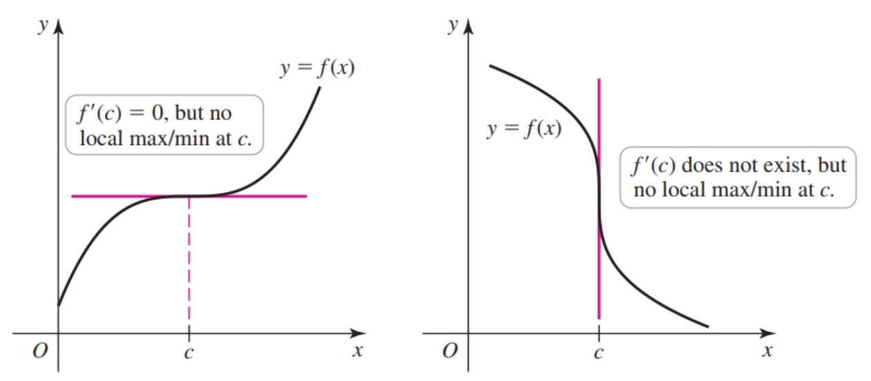
Therefore, critical points are candidates for the location of local extreme values, but you must determine whether they actually correspond to local maxima or minima.
Suppose $f$ is continuous on an interval $I$ that contains exactly one local extremum at $c$. If a local maximum occurs at $c$, then $f(c)$ is the absolute maximum of $f$ on $I$. If a local minimum occurs at $c$, then $f(c)$ is the absolute minimum of $f$ on $I$.
Locating Absolute Extreme Values on a Closed Interval
- Locate the critical points $c$ in $(a, b)$, where $f′(c) = 0$ or $f′(c)$ does not exist. These points are candidates for absolute maxima and minima.
- Evaluate $f$ at the critical points and at the endpoints of $[a, b]$.
- Choose the largest and smallest values of $f$ from the previous step for the absolute maximum and minimum values, respectively
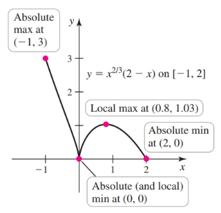
Given $g(x) = x^{2/3}(2 - x)$ on the interval $[-1, 2]$
- We first find the derivative to be $\frac{4 - 5x}{3x^{1/3}}$.
- $g'(0)$ is undefined (division by zero) and $0$ is in the domain of $g$, $x = 0$ is a critical point. $g'(x) = 0$ when $4 - 5x = 0$ so $x = \frac{4}{5}$ is also a critical point. These two points are candidates for the location of absolute extrema.
- Evaluating $g$ at endpoints and critical points shows that $g(-1) = 3, g(0) = 0, g(\frac{4}{5}) \approx 1.03, g(2) = 0$. Therefore, $g$ on the interval $[-1, 2]$ has its absolute maximum value at the endpoint $x = -1$ and its absolute minimum value at the critical point $x = 0$ and the endpoint $x = 2$.
Consider a function for which we must find the critical points:
$$ \begin{gather} f(x) = \frac{e^{2x}}{x -3} \end{gather} $$We find the derivative to be:
$$ \begin{gather} \begin{aligned} h'(x)&=\dfrac{d}{dx}\left[ \dfrac{e^{2x}}{x-3} \right] \\\\ &=\dfrac{(x-3)\cdot \dfrac{d}{dx}[e^{2x}]-e^{2x}\cdot \dfrac{d}{dx}[x-3]}{(x-3)^2} \\\\ &=\dfrac{(x-3)\cdot 2e^{2x}-e^{2x}\cdot 1}{(x-3)^2} \\\\ &=\dfrac{e^{2x}(2x-7)}{(x-3)^2} \end{aligned} \end{gather} $$$x = 3.5$ is a critical point, because $f'(3.5)$ is undefined. However, $x = 3$ is not a critical point because $f(3)$ is not defined.
Notice that trigonometric equations represent a special case:
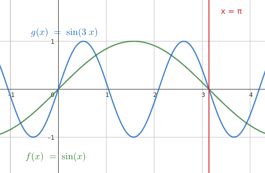
- there are three critical points on the interval $0 \le x \le \pi$
Finding the relative extremum points of:
$$ \begin{gather} f(x)=\dfrac{x^2}{x-1} \end{gather} $$we start with differentiating $f$:
$$ \begin{gather} f'(x)=\dfrac{x^2-2x}{(x-1)^2} \end{gather} $$The critical points of a function $f$ are the $x$-values, within the domain of $f$ for which $f'(x) = 0$ or where $f'$ is undefined. In addition to those, we should look for points where the function $f$ itself is undefined.
In our case, these points are $x = 0$, $x = 1$, and $x = 2$.
In a sign chart, we pick a test value at each interval that is bounded by the points we found and check the derivative’s sign on that value.
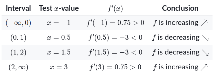
An extremum point would be a point where $f$ is defined and $f'$ changes signs.
In our case:
- $f$ increases before $x = 0$, decreases after it, and is defined at $x = 0$. So $f$ has a relative maximum point at $x = 0$.
- $f$ decreases before $x = 2$, increases after it, and is defined at $x = 2$. So $f$ has a relative minimum point at $x = 2$.
- $f$ is undefined at $x = 1$, so it doesn’t have an extremum point there.
Finding absolute extrema on a closed interval
Extreme value theorem tells us that a continuous function must obtain absolute minimum and maximum values on a closed interval. These extreme values are obtained, either on a relative extremum point within the interval, or on the endpoints of the interval.
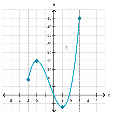
Let’s find, for example, the absolute extrema of $h(x)=2x^3+3x^2-12x$ over the interval $-3\leq x\leq 3$.
$h'(x)=6(x+2)(x-1)$ so our critical points are $x = -2$ and $x = 1$. They divide the closed interval $-3 \le x \le 3$ into three parts:
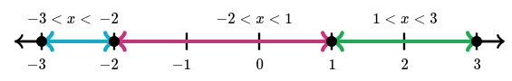
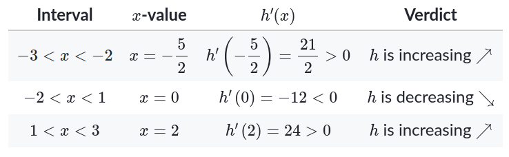
Now we look at the critical points and the endpoints of the interval:
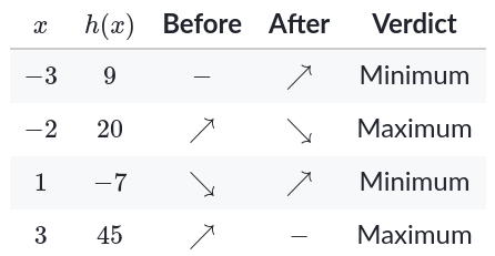
On the closed interval $-3 \le x \le 3$, the points $(-3, 9)$ and $(1, -7)$ are relative minima and the points $(-2, 20)$ and $(3, 45)$ are relative maxima.
$(1,-7)$ is the lowest relative minimum, so it’s the absolute minimum point, and $(3, 45)$ is the largest relative maximum, so it’s the absolute maximum point.
Finding absolute extrema on entire domain
Not all functions have an absolute maximum or minimum value on their entire domain. For example, the linear function $f(x) = x$ doesn’t have an absolute minimum or maximum (it can be as low or as high as we want).
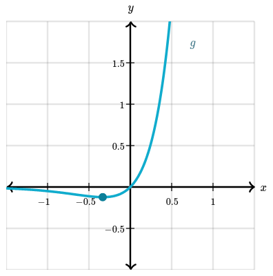
However, some functions do have an absolute extremum on their entire domain. Let’s analyze, for example, the function $g(x) = xe^{3x}$.
$g'(x)=e^{3x}(1+3x)$ , so our only critical point is $x = -\frac{1}{3}$.

Let’s imagine ourselves walking on the graph of $g$, starting all the way to the left (from $-\infty$) and going all the way to the right (until $+\infty$).
We will start by going down and down until we reach $x = -\frac{1}{3}$. Then, we will be forever going up. So $g$ has an absolute minimum point at $x = -\frac{1}{3}$. The function doesn’t have an absolute maximum value.
Other examples might have a restricted domain, e.g. the domain of $f(x) = \frac{\ln(x)}{x^2}$ is all real numbers such that $x \gt 0$.
Concavity
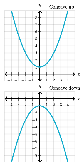
Graphically, a graph that’s concave up has a cup shape, $\cup$, and a graph that’s concave down has a cap shape, $\cap$.
Concavity relates to the rate of change of a function’s derivative. A function $f$ is concave up (or upwards) where the derivative $f'$ is increasing. This is equivalent to the derivative of $f'$, which is $f''$, being positive. Similarly, $f$ is concave down (or downwards) where the derivative $f'$ is decreasing (or equivalently, $f''$ is negative).
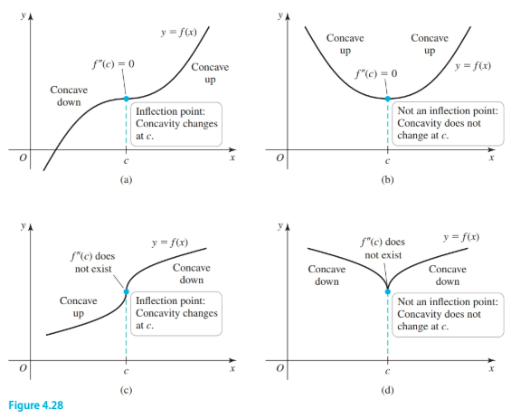
Inflection points (or points of inflection) are points where the graph of a function changes concavity (from $\cup$ to $\cap$ or vice versa).
$f''$ can be used determine concavity and inflection points of $f'$.
Suppose that $f$ exists on an open interval $I$.
- If $f'' > 0$ on $I$, then $f$ is concave up on $I$ (the slope of $f'$ is increasing on $I$)
- If $f'' < 0$ on $I$, then $f$ is concave down on $I$ (the slope of $f'$ is decreasing on $I$).
- If $f''(c) = 0$ or does not exist, then $c$ is a candidate for an inflection point ($f$ goes from concave up to concave down or vice versa)
Example
Given the following:
$$ \begin{gather} f(x) = 3x^4 - 4x^3 - 6x^2 + 12 x + 1\\ f'(x) = 12(x + 1)(x - 1)^2\\ f''(x) = 12(x - 1)(3x + 1) \end{gather} $$We see that $f''(x) = 0$ at $x = 1$ and $x = -\frac{1}{3}$. The points are candidates for inflection points. We use a sign graph to determine whether a sign change occurs which would indicate a change in concavity:
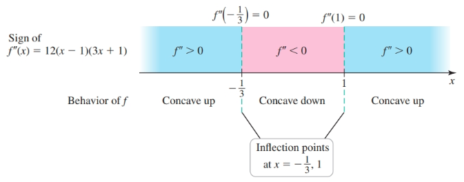
We see that the sign of $f''$ changes at $x = -\frac{1}{3}$ and at $x = 1$, so these are inflection points
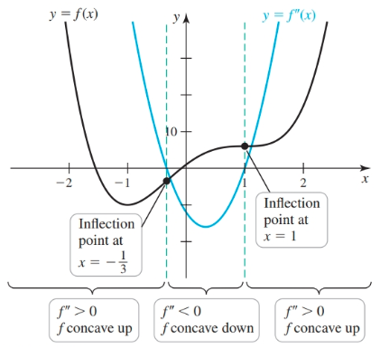
We can see the relationship between a function and its first and second derivative.
- $f'(x)$ reports the slope of $f(x)$
- $f''(x)$ reports inflection points.
The Second Derivative Test
Use the Second Derivative Test to identify local maxima and minima.
Suppose that $f′′$ is continuous on an open interval containing $c$ with $f′(c) = 0$.
- If $f′′(c) > 0$, then $f$ has a local minimum at $c$.
- If $f′′(c) < 0$, then $f$ has a local maximum at $c$.
- If $f′′(c) = 0$, then the test is inconclusive; $f$ may have a local maximum, local minimum, or neither at $c$.
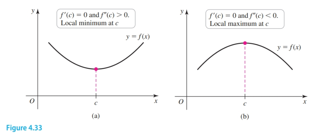
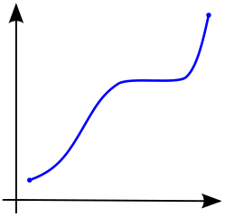
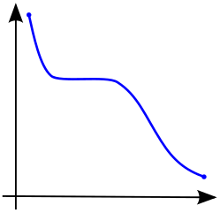
Notice the relationship between these functions and their first and second derivatives:
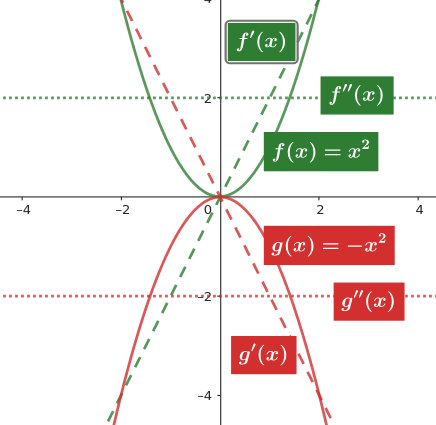
- for $f(x)$ $f'(0) = 0$ and $f''(0) \gt 0$
- for $g(x)$ $g'(0) = 0$ and $g''(0) \lt 0$
Graphing Derivatives
- Identify the domain or interval of interest e.g. $(-\infty, \infty)$ or restricted?
- Exploit symmetry an odd function such as $x^3$ is such that the third quadrant resembles the first quadrant rotated $180^\circ$, and an even function such as $x^2$ is mirrored about the $y$-axis.
- Find the first derivative, critical points, and where it is increasing/decreasing.
- Find the second derivative, inflection points, and where it is concave up/concave down.
- Identify extreme values.
- Locate all asymptotes and determine end behavior.
- Find the intercepts.
- Choose an appropriate window and plot a graph. It may be helpful to graph about a 1-dimensional first indicating points of inflection and critical points, and symbolically indicating increasing/decreasing intervals and concavity.
Example
Optimization Problems
Finding minima maxima of functions in the real world.
Example
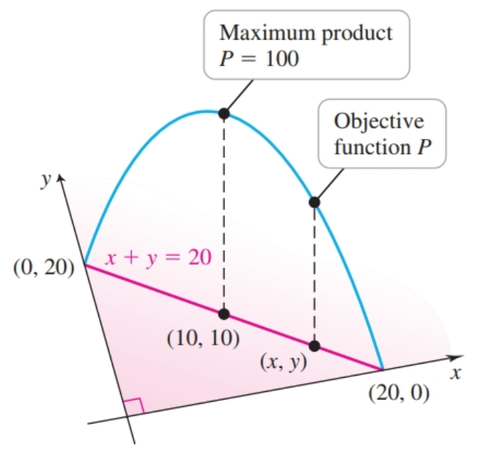
Find a pair of real numbers $x$ and $y$ between $0$ and $20$ with the property that their sum is $20$, that is, $x + y = 20$. Of all possible pairs, which has the greatest product? The condition that $x + y = 20$ is called a constraint. The quantity we wish to maximize (or minimize) is called the objective function; in this case, the objective function is the product $P = xy$.
To solve this do the following:
- Use the constraint to express the objective function $P = xy$ in terms of a single variable:
The objective function becomes $P = x(20 - x) = 20x - x^2$.
- To maximize $P$, we first find the critical points by solving $P'(x) = 20 - 2x = 0$ to obtain the solution $x = 10$
- Next we check endpoints and critical points. Because $P(0) = P20 = 0$ and $P(10) = 100$, we conclude that $P$ has its absolute maximum value at $x = 10$. By the constraint $x + y = 20$, the numbers with the greatest product are $x = y = 10$, and their product is $P = 100$.
Example
What is the smallest possible sum of squares of two numbers, if their product is -16?
So, we have two numbers $x$ and $y$ such that $x \cdot y = -16$, and we want to find the minimum of $f(x) = x + y$.
First, we must get $y$ in terms of $x$.
$$ \begin{gather} x \cdot y = -16\\ x = \frac{-16}{y} \end{gather} $$Next, we use the strategy for finding minima.
We find that $x = \pm 4$.
When $x = 4$, $y=-16/4 = 4$.
And, we find that the minimum of $f(x)$ is $f(4)$
Example
You are making a box by cutting away $x$ by $x$ squares from the corners of a piece of cardboard and folding the sides up:
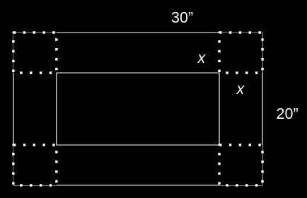
How do we find $x$ such that the volume is maximized?
The equation is:
$$ \begin{gather} v(x) = x \times 20 - 2x \times 30 - 2x \end{gather} $$We see that $x$ can’t be zero – we would make no folds at all! And, $x$ cannot be $10$ because then the width would be $0$.
So, we know $0 \lt x \lt 10$.
Expanding the original equation we get:
$$ \begin{gather} v(x) = 4x^3 - 100x^2 + 600x \end{gather} $$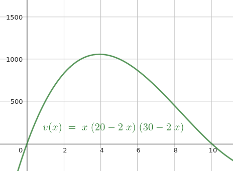
And, now we use the strategy for finding the maximum, which gives us $x = 3.92$.
Example
You run a shoe factory. Your formula for revenue is $r(x) = 10x$ (LHS in the thousands of dollars and RHS in thousands of pairs of shoes) and your cost is $x^3 - 6x^2 + 15x$. What is your profit and how many shoes should you produce to maximize profit? The formula for profit is $p(x) = r(x) - c(x)$. So, we have:
$$ \begin{gather} p(x) = 10x - (x^3 - 6x^2 + 15x)\\ = -x^3 + 6x^2 - 5x\\ = -x(x - 5)(x - 1) \end{gather} $$The least amount of shoes we can produce is $0$. Further, if we produce less than $1$ or more than $5$ our profit falls below $0$. Next, we use the strategy for finding the maximum to find a maximum of $3.528$ or $3,528$ pairs of shoes. Manufacturing this amount yields a profit of $p(3,528) = $$13,128$.
Example
A rectangular storage container with an open top needs to have a volume of 10 cubic meters. The length of its base is twice the width. Material for the base costs $10 per square meter. Material for the sides costs $6 per square meter. Find the cost of the material for the cheapest container.
First, we draw a picture.
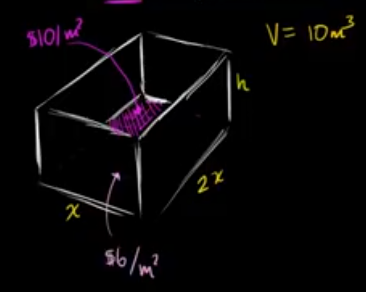
Next, we find our equations.
For the cost of the base we have:
$$ \begin{gather} f(x) = 10 \cdot x \cdot 2x \end{gather} $$The total cost of the sides is going to be:
$$ \begin{gather} g(x) = 6 \times (2xh) \times (xh) \end{gather} $$Therefore, our total cost can be determined with the following equation:
$$ \begin{gather} c(x) = (10 \cdot x \cdot 2x) + (6 \times (2xh) \times (xh)) = 20x^2 + 36xh \end{gather} $$Notice that we need find $h$ in terms of $x$. We know that the volume has to be $10\text{m}^3$.
$$ \begin{gather} 10 = 2x \cdot x \cdot h\\ h = \frac{5}{x^2} \end{gather} $$For our cost, we now have:
$$ \begin{gather} c(x) = 20x^2 + 180x^{-1} \end{gather} $$Next, we use the strategy to find the minimum. With $x = 0$ we’ve no base so our $x > 0$. We find $x \approx 1.65$ minimizes the cost. So, our cost will be $c(1.65) = 20 \times 1.65^2 + 180 / 1.65 \approx \$163.54$
Related Rates
Whenever ever you hear rate of change for some $f(x)$, e.g. rate of change of $y$ with respect to $x$, immediately recall that this is a derivative:
$$ \begin{gather} \frac{dy}{dx} \end{gather} $$If you need to put this in an equation, you can use or substitute in its value as needed.
Related rate problems relate two or more rates of change to each other. Maybe we want relate the rate of change of the side of a triangle given the related rate for another triangle, for example. One of the keys to solving these types of problems is finding an equation that relates the properties whose rates of change are relevant to the problem. Sometimes, an equation that relates properties will relate properties to a fixed value, e.g. $100 = x + y$, and other times this is not appropriate. Other times, the properties may relate to each other: $x/y = (10 + x)/20$.
Let’s say you drop a pebble in water and you find that the change in radius of the ripple is $3 \text{cm}/\text{s}$. In other words, we have the following derivative:
$$ \begin{gather} \frac{dr}{dt} = 3 \text{cm}/\text{s} \end{gather} $$This holds for any value of $t$.
We are also given that $r(t_0) = 8$. How can we find the instantaneous rate of change in area $A(t)$ of the ripple with respect to time at time $t_0$? We are looking for $A'(t_0)$.
$$ \begin{gather} \frac{dA}{dt} \end{gather} $$We can relate radius and area to each other with the following formula:
$$ \begin{gather} A = \pi r^2 \end{gather} $$Since we don’t have the explicit formulas for $A(t)$ and $r(t)$, we will use implicit differentiation:
$$ \begin{gather} A(t)&=\pi [r(t)]^2 \\\\ \dfrac{d}{dt}[A(t)]&=\dfrac{d}{dt}\Bigl[\pi [r(t)]^2\Bigr] \\\\ \goldD{A'(t)}&=2\pi\blueD{r(t)}\greenD{r'(t)} \end{gather} $$- Notice that we express the radius and area as a function of time and we use the chain rule on the right side.
We can substitute $r(t_0) = 8$ and $r'(t_0) = 3$ into that equation:
$$ \begin{gather} \goldD{A'(t_0)}&=2\pi\blueD{r(t_0)}\greenD{r'(t_0)} \\\\ &=2\pi(\blueD 8)(\greenD 3) \\\\ &=48\pi \end{gather} $$The area is increasing at a rate of $48\pi$ square centimeters per second.
Two cars are driving towards an intersection from perpendicular directions. The first car’s velocity is $50 \text{km}{h}$ and the second car’s velocity is $90 \text{km}/\text{h}$. At a certain instant $t_0$, the first car is a distance $x(t_0)$ of $0.5 \text{km}$ from the intersection and the second car is a distance $y(t_0)$ of $1.2 \text{km}$ from the intersection. What is the formula we can use to find the rate of change of the distance $d(t)$ between the cars at that instant?
First, we need to relate everything.
Using the Pythagorean theorem we can find the following relationship:
$$ \begin{gather} d(t) = \sqrt{x(t)^2 + y(t)^2}\\ d(t)^2 = x(t)^2 + y(t)^2 \end{gather} $$We begin finding the rate of change of distance at time $t$ with the following equation:
$$ \begin{gather} \frac{d}{dt}[d(t)] = \frac{d}{dt}[x(t)^2 + y(t)^2] \end{gather} $$A $20$-meter ladder is leaning against a wall. The distance $x(t)$ between the bottom of the ladder and the wall is increasing at a rate of $3$ meters per minute. At a certain instant $t_0$, the top of the ladder is a distance $y(t_0)$ of $15$ meters from the ground. What is the rate of change of the angle $\theta(t)$ between the ground and the ladder?
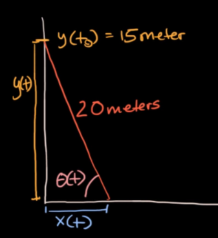
We can use trigonometry. We can relate the quantities with the following equation:
$$ \begin{gather} x(t) = 20 \cos(\theta(t))\\ x'(t) = -20 \sin(\theta(t)) \cdot \theta'(t)\\ 3 = -20\left(\frac{y(t_0)}{20}\right) \cdot \theta'(t)\\ = -15 \cdot \theta'(t)\\ \theta'(t) = \frac{-1}{5} \frac{\text{radians}}{\text{minute}} \end{gather} $$Related rates (multiple rates)
The side of the base of a square pyramid is increasing at a rate of $6$ meters per minute and the height of the pyramid is decreasing at a rate of $1$ meter per minute.
At a certain instant, the base’s side is $3$ meters and the height is $9$ meters.
What is the rate of change of the volume of the pyramid at that instant (in cubic meters per minute)?
First we find a way to relate all of these. The equation for the volume of a square pyramid with base side $s$ and height $h$ is
$$ \begin{gather} V = \dfrac{1}{3}s^2h \end{gather} $$Now we differentiate with respect to time ($t$):
$$ \begin{gather} \frac{d}{dt}[V] = \frac{1}{3} \frac{d}{dt}[s^2] \frac{d}{dt}[h]\\ = \frac{1}{3} = \frac{1}{3} \left[ (2s \cdot 6 \cdot h) + (1 \cdot (-1) \cdot s^2)\right] \end{gather} $$Notice that we’ve used the chain rule and them the product rule. After substituting in the variables we get $105$ for the answer.
We have a cone that is $4$ cm high and a base diameter that is also $4$ cm. We are filling it with water at a rate of $1 \text{cm}^3/\text{s}$. The height of the water in the cone is currently $2$ cm. What is the rate that the height changes at this instant?
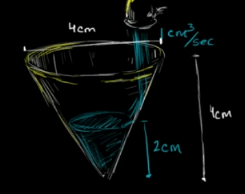
First, we need an equation relating all of the quantities:
$$ \begin{gather} V = \frac{1}{3}A \cdot h\\ = \frac{1}{3}\pi r^2 h \end{gather} $$Now, we work on finding the rate of the change of height $h$ with respect to time:
$$ \begin{gather} \frac{d}{dt}[V] = \frac{1}{3}\pi \frac{d}{dt}[r^2] \cdot \frac{d}{dt}[h]\\ 1 = \frac{1}{3}\pi \frac{dr}{dt}2rh + \frac{dh}{dt}(1)(r^2)\\ \end{gather} $$Notice that we are stuck because we cannot solve $\frac{dh}{dt}$ while $\frac{dr}{dt}$ is also unknown.
The key insight here is relate height and radius since we are given the diameter and the height (they are equal):
$$ \begin{gather} r = \frac{1}{2}h \end{gather} $$Now, we can rewrite our equation for volume as:
$$ \begin{gather} V = \frac{1}{3}\pi (\frac{1}{2}h)^2h\\ = \frac{1}{12}\pi h^3 \end{gather} $$Now, we differentiate:
$$ \begin{gather} 1 = \frac{1}{12}\pi \frac{dh}{dt}3h^2\\ = \frac{1}{12}\pi \frac{dh}{dt}3(2)^2\\ \end{gather} $$Solving the equation we get a rate of change for height of $\frac{1}{\pi} \frac{\text{cm}}{\text{s}}$.
Another Example
The volume of a sphere is increasing at a rate of $25\pi$ cubic meters per hour. At a certain instant, the volume is $\frac{32\pi}{3}$ cubic meters. What is the rate of change of the surface area of the sphere at that instant (in square meters per hour)?
We have the following equations:
- The surface area of a sphere with radius $r$ is $4 \pi r^2$.
- The volume of a sphere with radius $r$ is $\frac{4}{3} \pi r^3$.
Let
- $r(t)$ denote the sphere’s radius at time $t$,
- $V(t)$ denote the sphere’s volume at time $t$, and
- $S(t)$ denote the sphere’s surface area at time $t$
We are given $V'(t) = 25 \pi$, and we are give $V(t_0) = \frac{32\pi}{3}$ for a specific time $t_0$. We want to find $S'(t_0)$.
We can relate $S(t)$ to $r(t)$ through the surface area formula. So, we have:
$$ \begin{gather} S'(t) = 8\pi r(t)r'(t) \end{gather} $$To solve this we need $r'(t)$.
Knowing volume at time $t_0$ and the formula for volume, we can find $r = 2$. Knowing $V'(t)$ and $r(t_0)$, we can now find $r'(t)$:
$$ \begin{gather} V'(t_0) = 4 \pi[r(t_0)]^2 r'(t_0)\\ 25 \pi = 4 \pi(2)^2 r'(t_0)\\ \frac{25}{16} = r'(t_0) \end{gather} $$Now, we can plug this into the equation for $S'(t_0)$:
$$ \begin{gather} S'(t_0) = 8 \pi r(t_0) r'(t_0)\\ = 8 \pi(2) \left(\frac{25}{16}\right)\\ = 25 \pi \end{gather} $$Given the following:
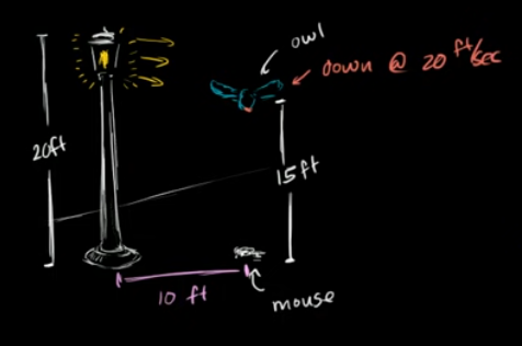
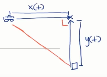
We know that the velocity of the owl is $\frac{dy}{dt} = 20 \text{ft}/\text{sec}$ down. What is the rate of change of the length of the shadow owl to the mouse?
The key to this problem is observing that we have similar triangles at work.
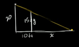
Therefore, we can relate $x$ and $y$ in the following way:
$$ \begin{gather} \frac{x}{y} = \frac{10 + x}{20}\\ 20x = 10y + xy \end{gather} $$We can solve for $x$ given $y = 15$:
$$ \begin{gather} 20x = 10(15) + 15x\\ 5x = 150\\ x = 30 \end{gather} $$Now, we can find $dx/dt$:
$$ \begin{gather} 20x = 10y + xy\\ 20 dx/dt = 10dy/dt + \frac{dx}{dt}y + \frac{dy}{dt}x\\ = 10(-20) + \frac{dx}{dt}(15) + (-20)(30)\\ = - 200 - 600 + \frac{dx}{dt}(15)\\ 5 dx/dt = -800\\ dx/dt = -160 \frac{\text{ft}}{\text{sec}} \end{gather} $$Suppose we have a balloon that is floating upwards:
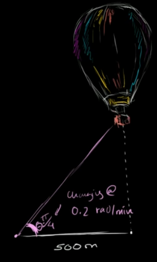
The balloon remains a fixed distance of $500\text{m}$ and we have that the angle grows in the instant at a rate of $0.2 \frac{\text{radians}}{\text{sec}}$. What is the velocity of the balloon in the upward direction ($\frac{dh}{dt}$)?
We have the following relationship:
$$ \begin{gather} \tan(\theta) = \frac{h}{500}\\ \frac{d}{dt}[\tan(\theta)] = \frac{d}{dt}[\frac{h}{500}]\\ \frac{d(\tan(\theta))}{dt} = \frac{1}{500}\frac{dh}{dt}\\ \frac{dh}{dt} = 0.2 \times \sec^2(\frac{\pi}{4}) \times 500\\ = 200 \frac{\text{m}}{\text{s}} \end{gather} $$Linear Approximation
Note that if you zoom in close enough on a point on a non-linear function that is differentiable the function looks linear.
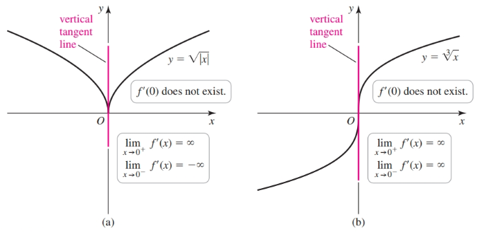
Here is a function that is not differentiable at $(0, 0)$, and so it does not appear linear at that point:
And, here is another function such that the tangent line at the point is a vertical line:
You can use the line tangent to a non-linear function to approximate nearby values. This technique is known as linear approximation or local linearization
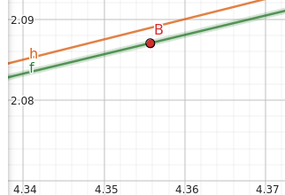
For example, how could you estimate $\sqrt{4.36}$ without using a calculator? This is equivalent to finding $f(4.36)$ where $f(x) = \sqrt{x} = x^{1/2}$.
We know that $f(4) = 2$. It turns out that we can draw a line tangent to $f(x)$ where $x = 4$ to approximate $f(4.36)$:
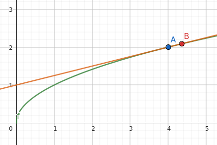
We have the $f(4)$, and $f'(4)$ gives the slope of a line $g(x)$, which at $g(4.36)$ approximates $f(4.36)$
Formally, we have:
$$ \begin{gather} L(x) = f(4) + f'(4)(x - 4) \end{gather} $$- Note that we have $f(4)$ plus the distance between $x$ and $4$ scaled by slope of the line tangent to $f(4)$
For $L(4.36)$, we have:
$$ \begin{gather} L(4.36) = f(4) + f'(4)(4.36 - 4)\\ = 2 + \frac{1}{4}(0.36)\\ = 2.09 \approx f(4.36) \end{gather} $$We can see that $L(x)$ overestimates $f(x)$ in this case:
Assume $f$ is differentiable on an interval containing the point $a$. The slope of the line tangent to the curve at the point $(a, f(a))$ is $f'(a)$. Therefore, an equation of the tangent line is
$$ \begin{gather} y - f(a) = f'(a)(x - a) \end{gather} $$or
$$ \begin{gather} y = \underbrace{f(a) + f'(a)(x - a)}_{L(x)} \end{gather} $$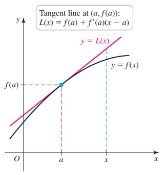
This tangent line represents a new function $L$ that we call the linear approximation to $f$ at the point $a$. If $f$ and $f'$ are easy to evaluate at $a$, then the value of $f$ at points near $a$ is easily approximated using the linear approximation $L$ i.e.:
$$ \begin{gather} f(x) \approx L(x) = f(a) + f'(a)(x - a), \text{ for } x \text{ in } I \end{gather} $$When the tangent line lies above the graph the approximation is an overestimate, otherwise, it is an underestimate.
We can find a measure of the error with $|L(x) - f(x)|$ and as a percentage with $\frac{100 \cdot |L(x) - f(x)|}{|f(x)|}$.
Linear Approximation and Concavity
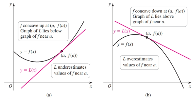
A large value of $|f''(a)|$ (large curvature) means that near $(a, f(a))$, the slope of the curve changes rapidly and the graph of $f$ separates quickly from the tangent line. A small value of $f''(a)$ (small curvature) means the slope of the curve changes slowly and the curve is relatively flat near $(a, f(a))$; therefore, the curve remains close to the tangent line. As a result, absolute errors in linear approximation are larger when $f''(a)$ is large.
Variation on Linear Approximation
We can rewrite the formula for linear approximation as:
$$ \begin{gather} f(x) \approx f(a) + f'(a)(x - a)\\ \underbrace{f(x) - f(a)}_{\Delta y} \approx f'(a)\underbrace{(x - a)}_{\Delta x}\\ \Delta y \approx f'(a) \Delta x \end{gather} $$This allows us to approximate the change $\Delta y$ in the dependent variable when $x$ changes from $a$ to $a + \Delta x$.
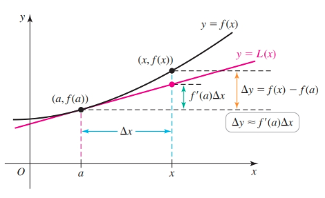
Suppose $f$ is differentiable on an interval $I$ containing the point $a$. The change in the value of $f$ between two points $a$ and $a + \Delta x$ is approximately $\Delta y \approx f'(a) \Delta x$, where $a + \Delta x$ is in $I$.
Differentials
Let $f$ be differentiable on an interval containing $x$. A small change in $x$ is denoted by the differential $dx$. The corresponding change in $f$ is approximated by the differential $dy = f'(x) dx$; that is
$$ \begin{gather} \Delta y = f(x + dx) - f(x) \approx dy = f'(x) dx \end{gather} $$Consider a function $y = f(x)$ differentiable on an interval containing $a$. If the $x$-coordinate changes from $a$ to $a$ + $\Delta x$, the corresponding change in the function is exactly
$$ \begin{gather} \Delta y = f(a + \Delta x) - f(a) \end{gather} $$Using the linear approximation $L(x) = f(a) + f'(a)(x - a)$, the change in $L$ as $x$ changes from $a$ to $a + \Delta x$ is
$$ \begin{gather} \Delta L = L(a + \Delta x) - L(a)\\ = \underbrace{(f(a) + f'(a)(a + \Delta x - a))}_{L(a + \Delta x} - \underbrace{(f(a) + f'(a)(a - a))}_{L(a)} = f'(a) \Delta x \end{gather} $$To distinguish $\Delta y$ and $\Delta L$, we define two new variables called differentials. The differential $dx$ is simply $\Delta x$; the differential $dy$ is the change in the linear approximation, which is $\Delta L = f'(a) \Delta x$.
Using this notation,
$$ \begin{gather} \Delta L = \underbrace{dy}_{\text{same as } \Delta L} = f'(a) \Delta x = f'(a) \underbrace{dx}_{\text{ same as } \Delta x} \end{gather} $$Therefore, at the point $a$, we have $dy = f'(a) dx$. More generally, we replace the fixed point $a$ by a variable point $x$ and write
$$ \begin{gather} dy = f'(x) dx \end{gather} $$The notation for differentials is consistent with the notation for the derivative: If we divide both sides of $dy = f'(x) dx$ by $dx$, we have
$$ \begin{gather} \frac{dy}{dx} = \frac{f'(x)dx}{dx} = f'(x) \end{gather} $$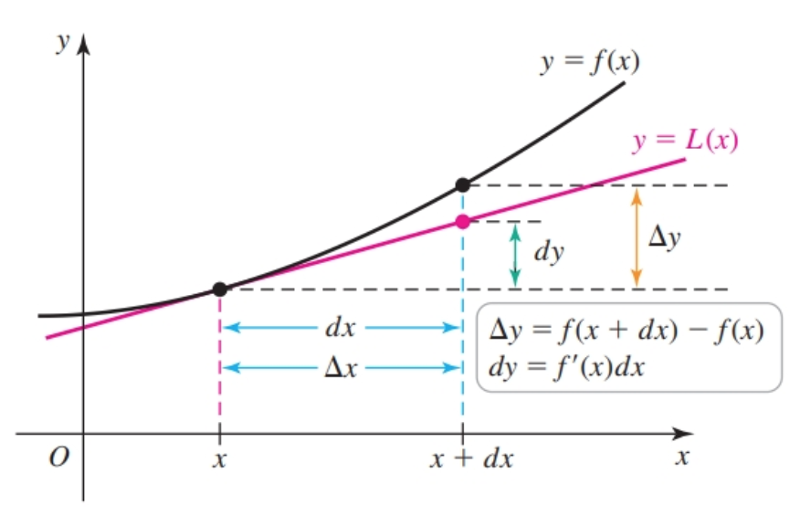
L’Hôpital’s Rule
Some limits, called indeterminate forms, cannot generally be evaluated using techniques such as direct substitution.
L’Hôpital’s rule helps us evaluate indeterminate limits of the form: $\frac{0}{0}$ or $\frac{\infty}{\infty}$.
In other words, it helps us find $\displaystyle\lim_{x\to c}\dfrac{u(x)}{v(x)}$, where $\displaystyle\lim_{x\to c}u(x)=\lim_{x\to c}v(x)=0$ (or, alternatively, where both limits are $\pm \infty$).
The rule essentially says that if the limit $\displaystyle\lim_{x\to c}\dfrac{u'(x)}{v'(x)}$ exists, then the two limits are equal:
$$ \begin{gather} \displaystyle\lim_{x\to c}\dfrac{u(x)}{v(x)}=\displaystyle\lim_{x\to c}\dfrac{u'(x)}{v'(x)} \end{gather} $$}
Suppose $f$ and $g$ are differentiable on an open interval $I$ containing $a$ with $g'(x) \ne 0$ on $I$ when $x \ne a$. If $\lim_{x \to a} f(x) = \lim_{x \to a} g(x) = 0$, then
$$ \begin{gather} \lim_{x \to a} \frac{f(x)}{g(x)} \end{gather} $$cannot be solved by direct substitution as the result will be $0 \div 0$. We represent this inderterminate form with $0/0$.
The following is also an indeterminate form:
$$ \begin{gather} \lim_{x \to \infty} \frac{x}{x + 1} \end{gather} $$This limit has the indeterminate form $\infty/\infty$ meaning that the numerator and denominator become arbitrarily large in magnitude as $x \to \infty$
Similarly,
$$ \begin{gather} \lim_{x \to c} \frac{f(x)}{g(x)} \end{gather} $$Is an indeterminate form where $\lim_{x \to c}f(x) = \pm \infty$ and $\lim_{x \to c}g(x) = \pm \infty$.
When given the indeterminate forms $0/0$ or $\infty/\infty$ we may find the limit with L’Hopital’s rule which makes use of derivatives, i.e. we use derivatives to find limits of indeterminate forms that cannot be solved conventionally.
Suppose $f$ and $g$ are differentiable on an open interval $I$ containing $a$ with $g'(x) \ne 0$ on $I$ when $x \ne a$. If $\lim_{x \to a} f(x) = \lim_{x \to a} g(x) = 0$, then
$$ \begin{gather} \lim_{x \to a} \frac{f(x)}{g(x)} = \lim_{x \to a} \frac{f'(x)}{g'(x)} \end{gather} $$provided the limit on the right exists (or is $\pm \infty$). The rule also applies if $x \to a$ is replaced with $x \to \pm \infty$, $x \to a^+$, or $x \to a^-$.
Likewise, suppose $f$ and $g$ are differentiable on an open interval $I$ containing $a$, with $g'(x) \ne 0$ on $I$ when $x \ne a$. If $\lim_{x \to a} f(x) = \pm \infty$ and $\lim_{x \to a} g(x) = \pm \infty$, then
$$ \begin{gather} \lim_{x \to a} \frac{f(x)}{g(x)} = \lim_{x \to a} \frac{f'(x)}{g'(x)} \end{gather} $$provided the limit on the right exists (or is $\pm \infty$). The rule also applies for $x \to \pm \infty, x \to a^+, x \to a^-$.
Given the $0/0$ indeterminate form $\lim_{x \to 1} \frac{x^3 + x^2 - 2x}{x - 1}$ we can evaluate with L’Hopital’s rule to find a solution of: $\lim_{x \to 1} \frac{3x^2 + 2x - 1}{1} = 3$
One thing to notice about these indeterminate forms is that they are of the form $f(x)/g(x)$. If we have an expression such as:
$$ \begin{gather} \lim_{x \to 0^+} x^4 \ln (x) \end{gather} $$We want to rewrite it as:
$$ \begin{gather} \lim_{x \to 0^+} \frac{\ln (x)}{x^{-4}} \end{gather} $$L’Hopital’s rule can be applied multiple times as applying the rule may result in an indeterminate form.
L’Hopital’s Rule for $\infty/\infty$ applied three times (until the form is not indeterminate):
$$ \begin{gather} \lim_{x \to \infty} \frac{4x^3 - 6x^2 + 1}{2x^3 - 10x + 3}\\ \lim_{x \to \infty} \frac{12x^2 - 12x}{6x^2 - 10}\\ \lim_{x \to \infty} \frac{24x - 12}{12x}\\ \lim_{x \to \infty} \frac{24}{12} = 2 \end{gather} $$Challenging Problem
How do we solve for:
$$ \begin{gather} \lim_{x \to 1} \left( \frac{x}{x - 1} - \frac{1}{\ln x} \right) \end{gather} $$Unfortunately, we cannot solve the problem as the sum of $2$ separate limits, i.e.:
$$ \begin{gather} \lim_{x \to 1} \left( \frac{x}{x - 1} \right) - \lim_{x \to 1} \left( \frac{1}{\ln x} \right) \end{gather} $$Instead, we must proceed this way (finding a common denominator):
$$ \begin{gather} \lim_{x \to 1} \left( \frac{ x \ln x - (x - 1)}{(x - 1)\ln x} \right) \end{gather} $$Applying L’Hopital’s Rule gives us a limit of:
$$ \begin{gather} \frac{1}{2} \end{gather} $$$0 \cdot \infty$ and $\infty - \infty$
Other indeterminate forms cannot be evaluated with L’Hôpital’s Rule, but must first be recast to either $0/0$ or $\infty/\infty$.
Limits of the form $\lim_{x \to a} f(x) g(x)$, where $\lim_{x \to a} f(x) = 0$ and $\lim_{x \to a} g(x) = \pm \infty$ are indeterminate; such limits are denoted $0 \cdot \infty$.
Limits of the form $\lim_{x \to a} (f(x) - g(x))$, where $\lim_{x \to a} f(x) = \infty$ and $\lim_{x \to a} g(x) = \infty$, are indeterminate forms that we denote $\infty - \infty$.
Divide by the reciprocal
$$ \begin{gather} \underbrace{\lim_{x \to \infty} x^2 \sin(\frac{1}{4x^2})}_{\infty \cdot 0 \text{ form }} = \underbrace{\lim_{x \to \infty} \frac{\sin(\frac{1}{4x^2})}{\frac{1}{x^2}}}_{\text{recast in } 0/0 \text{ form }} \end{gather} $$Convert the Limit
Occasionally, it helps to convert a limit as $x \to \infty$ to a limit as $t \to 0^+$ (or vice versa) by a change of variables. To evaluate $\lim_{x \to \infty} f(x)$, we define $t = 1/x$ and note that as $x \to \infty$, $t \to 0^+$. Then
$$ \begin{gather} \lim_{x \to \infty} f(x) = \lim_{t \to 0^+} f\left(\frac{1}{t}\right) \end{gather} $$Here is an example:
$$ \begin{gather} \lim_{x \to \infty} \frac{1 - \sqrt{1 - 3/x}}{1/x} = \lim_{t \to 0^+} \frac{1 - \sqrt{1 - 3t}}{t}\\ = \lim_{t \to 0^+} \frac{\frac{3}{2\sqrt{1 - 3t}}}{1}\\ = \frac{3}{2} \end{gather} $$L’Hôpital’s Rule for $\infty - \infty$
Given $\lim_{x \to \infty} (x - \sqrt{x^2 - 3x})$
- Factor out $x$:
This is now in the indeterminate form $0/0$
- Substitute the expression $1/x$ for $t$ i.e. $t = 1/x$:
$1^\infty, 0^0, \infty^0$
The indeterminate forms $1^\infty, 0^0, \infty^0$ all arise in limits of the form $\lim_{x \to a} f(x)^{g(x)}$, where $x \to a$ could be replaced with $x \to a^\pm$ or $x \to \pm \infty$.
We use the natural logarithm to process these indeterminate forms. The inverse relationship between $\ln x$ and $e^x$ says that $f^g = e^{g \ln f}$, so we first write:
$$ \begin{gather} \lim_{x \to a} f(x)^{g(x)} = \lim_{x \to a} e^{g(x) \ln f(x)} \end{gather} $$By the continuity of the exponential function, we switch the order of the limit and the exponential function:
$$ \begin{gather} \lim_{x \to a} e^{g(x) \ln f(x)} = e^{\lim_{x \to a} g(x) \ln f(x)} = \exp[\lim_{x \to a} g(x) \ln f(x)] \end{gather} $$provided $\lim_{x \to a} g(x) \ln f(x)$ exists.
Next, Analyze $L = \lim_{x \to a} g(x) \ln f(x)$. This limit can be put in the form $0/0$ or $\infty/\infty$.
When $L$ is finite, $\lim_{x \to a} f(x)^{g(x)} = e^L$. If $L = \infty$ or $-\infty$, then $\lim_{x \to a} f(x)^{g(x)} = \infty$ or $\lim_{x \to a} f(x)^{g(x)} = 0$, respectively.
Note the following results:
- For $1^{\infty}$, $L$ has the form $\infty \cdot \ln 1 = \infty \cdot 0$
- For $0^0$, $L$ has the form $0 \cdot \ln 0 = 0 \cdot -\infty$.
- For $\infty^0$, $L$ has the form $0 \cdot \ln \infty = 0 \cdot \infty$
Example
Consider the following:
$$ \begin{gather} \lim_{x \to 0^+} (\sin x)^{\frac{1}{\ln x}} \end{gather} $$Substituting in $0$ gives us:
$$ \begin{gather} 0^0 \end{gather} $$We can make progress using the natural logarithm:
$$ \begin{gather} y(x) = (\sin x)^{\frac{1}{\ln x}}\\ \ln y = \ln (\sin x)^{\frac{1}{\ln x}}\\ = \frac{1}{\ln x} \ln (\sin x)\\ = \frac{\ln(\sin x)}{\ln x} \end{gather} $$Let’s now take the limit of this:
$$ \begin{gather} \lim_{x \to 0^+} \frac{\ln (\sin x)}{\ln x} \end{gather} $$Substituting in $0$ gives us:
$$ \begin{gather} \frac{ -\infty}{-\infty} \end{gather} $$With this indeterminate form, We can now use L’Hopital’s Rule:
$$ \begin{gather} \lim_{x \to 0^+} \frac{\frac{\cos x}{\sin x}}{\frac{1}{x}}\\ = \lim_{x \to 0^+} \frac{x \cos x}{\sin x} \end{gather} $$Substituting in $0$ gives us $\frac{0}{0}$. We can separate the limit, like so:
$$ \begin{gather} \left(\lim_{x \to 0^+} \frac{x}{\sin x}\right)\left(\lim_{x \to 0^+} \cos x \right) \end{gather} $$Substituting in $0$ We get:
$$ \begin{gather} \frac{0}{0} \times 1 \end{gather} $$So, we apply L’Hopital’s Rule again:
$$ \begin{gather} \lim_{x \to 0^+} \frac{1}{\cos(x)} = 1 \end{gather} $$Therefore, for the limit of second equation we have:
$$ \begin{gather} \lim_{x \to 0^+} (\ln y) = 1 \end{gather} $$If $\ln y \to 1$, then $y \to e$, because $\ln(e) = 1$. Therefore, for our original limit we have:
$$ \begin{gather} \lim_{x \to 0^+} (\sin x)^{\frac{1}{\ln x}} = e \end{gather} $$Using L’Hôpital’s Rule with Nonlinear Functions
If $f$ and $g$ are not linear functions, we replace them with their linear approximations at $a$. Near $x = a$, we have
$$ \begin{gather} \frac{f(x)}{g(x)} \approx \frac{f'(a)(x - a)}{g'(a)(x - a)} = \frac{f'(a)}{g'(a)} \end{gather} $$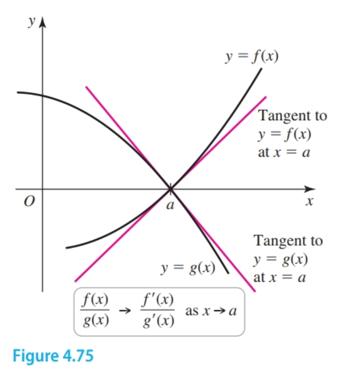
Therefore, the ratio of the functions is well approximated by the ratio of the derivatives. In the limit as $x \to a$, we again have
$$ \begin{gather} \lim_{x \to a} \frac{f(x)}{g(x)} = \lim_{x \to a} \frac{f'(x)}{g'(x)} \end{gather} $$Proof of Special Case of l’Hopital’s Rule
This is not a full proof of the rule, but it gives an intuition for how it works.
If we have the following:
- $f(a) = 0$, $f'(a)$ exists
- $g(a) = 0$, $g'(a)$ exists
Then l’Hopital’s Rule gives us the following:
$$ \begin{gather} \lim_{x \to a} \frac{f(x)}{g(x)} = \frac{f'(a)}{g'(a)} \end{gather} $$Recall the definition of a limit, and what we have is:
$$ \begin{gather} f'(a) = \lim_{x\to a}\frac{f(x) - f(a)}{x - a} \end{gather} $$And, similarly, for $g'(a)$
$$ \begin{gather} g'(a) = \lim_{x\to a}\frac{g(x) - g(a)}{x - a} \end{gather} $$And, therefore, we have:
$$ \begin{gather} \frac{f'(a)}{g'(a)} = \frac{\lim_{x\to a}\frac{f(x) - f(a)}{x - a}}{\lim_{x \to a}\frac{f(x) - f(a)}{x - a}}\\ = \lim_{x\to a} \frac{f(x) - f(a)}{g(x) - g(a)}\\ = \lim_{x \to a} \frac{f(x)}{g(x)} \end{gather} $$Rolle’s Theorem
Let $f$ be continuous on a closed interval $[a, b]$ and differentiable on $a$, $b$ with $f(a) = f(b)$. There is at least one point $c$ in $(a, b)$ such that $f'(c) = 0$.
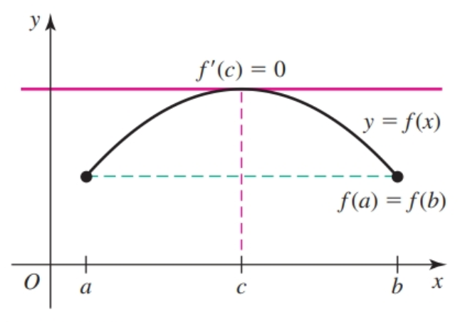
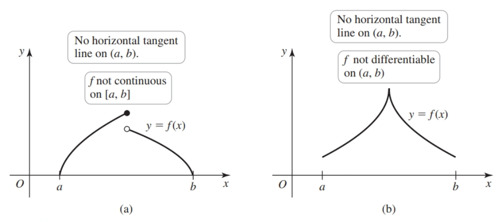
Rolle’s Theorem requires continuity because as function that is not continuous on $[a, b]$ may have identical values and still not have a horizontal tangent line at any point on the interval. Similarly, a function that is continuous on $[a, b]$ but not differentiable at a point of $(a, b)$ may also fail to have a horizontal tangent line.
Mean Value Theorem
Allows you to find $c$ between points $a$ and $b$ under certain conditions. It is similar to intermediate and extreme value theorems.
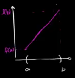
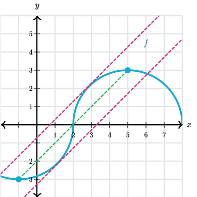
Given a function $f$ continuous over $[a, b]$ and differentiable over $(a, b)$ with a secant line passing through $(a, f(a))$ and $(b, f(b))$, there is a tangent line parallel to the secant line that passes through $c \in (a, b)$ whose slope we can derive with:
$$ \begin{gather} \frac{f(b) - f(a)}{b - a} = m_{\sec} = m_{\tan} = f'(c) \end{gather} $$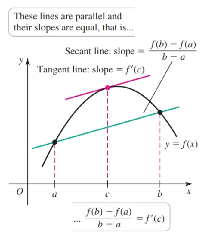
In other words, given an average change between $a$ and $b$ under the conditions specified, there is an equivalent instantaneous rate of change at $c$.
Knowing $f'(c)$, we can find $c$ algebraically.
Given the following polynomial (continuous everywhere and differentiable) and its derivative on the interval $[-2, 2]$:
$$ \begin{gather} f(x) = 2x^3 - 3x + 1\\ f'(x) = 6x^2 - 3 \end{gather} $$We find $f'(c)$ to be:
$$ \begin{gather} \frac{f(2) - f(-2)}{2 - (-2)} = 5 \end{gather} $$Now, we can solve for $c$ with:
$$ \begin{gather} 5 = 6c^2 - 3\\ c = \pm 2/\sqrt{3} \end{gather} $$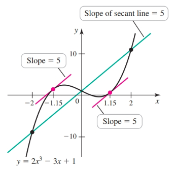
Why is differentiability over the interval important?
The function has a sharp turn between $x = a$ and $x = b$, so it’s not differentiable over $(a, b)$.
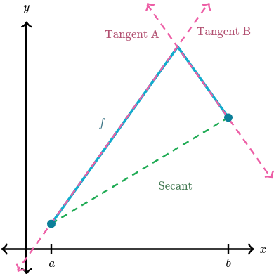
Indeed, the function has only two possible tangent lines, neither of which is parallel to the secant between $x = a$ and $x = b$.
Why is continuity at the edges important?
$g$ is not continuous at $x = b$.
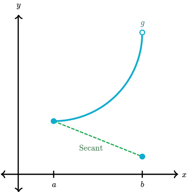
Notice how all of the possible tangent lines on the interval are necessarily increasing, while the secant line is decreasing. So there isn’t any tangent line that’s parallel to the secant line.
For the function below, MVT doesn’t apply over the interval $[-1, 5]$, even though there are actually two points in the interval $[-1, 5]$ where the tangent is parallel to the secant between the endpoints.
- Notice that the function is not differentiable at $f(2)$.
This goes to show that we can’t be certain about MVT unless the conditions of continuity and differentiability have been met
Consequences
- If $f$ is differentiable and $f'(x) = 0$ at all points of an interval $I$ i.e. $\frac{f(b) - f(a)}{b - a} = f'(c) = 0$, then $f$ is a constant function on $I$.
- If two functions have the property that $f'(x) = g'(x)$, for all $x$ of an interval $I$, then $f(x) - g(x) = C$ on $I$, where $C$ is a constant; that is, $f$ and $g$ differ by a constant. Recall that the derivative of a difference of two functions equals the difference of the derivatives so we can write $f'(x) - g'(x) = (f - g)'(x) = 0$
Newton’s Method
Given a function $f(x)$, we can find the roots of that function given an initial value and $f'(x)$. These roots may be the roots of a quadratic equation, infection points, etc.
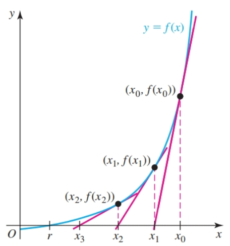
Suppose that $r$ is a root of $f$ i.e. $f(r) = 0$, and assume that $f$ is differentiable on some interval containing $r$. Suppose $x_0$ is an initial approximation to $r$. We can find a better approximation with these steps
- draw a line tangent to the curve $y = f(x)$ at the point $(x_0, f(x_0))$
- the point $(x_1, 0)$ at which the tangent line intersects the $x$-axis is found and $x_1$ becomes the new approximation to $r$.
- $x_1$ is used to approximate $x_2$, and so on until the desired $x_n$ is found
Given an approximation of $x_n$, we can find the next approximation ($x_{n + 1}$) with:
$$ \begin{gather} x_{n + 1} = x_n - \frac{f(x_n)}{f'(x_n)} \end{gather} $$- A general rule of thumb is that if two successive approximations agree to, say, seven digits, then those common digits are accurate (as an approximation to the root).
- or, you can calculate to the desired number of iterations
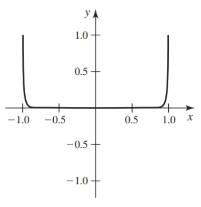
As the approximations $x_n$ approach the root, $f(x_n)$ should approach zero. The errror in $x_n$ is $|x_n - r|$. The quantity $f(x_n)$ is called a residual, and small residuals usually (but not always) suggest that the approximations have small errors and can give additional confidence that the approximations have small errors.
However, small residuals do not always imply small errors. The function shown below has a zero at $x = 0$ with a small residual of $0.5$ but a large error.
Newton’s method cannot be used if the $f'(x_n) = 0$ If $f'(x_n)$ is close to zero at any step then the method may converge slowly or fail to converge
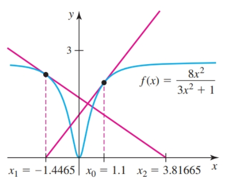
This is the case with $x_0 = 0.15$ and the function $\frac{8x^2}{3x^2 + 1}$.
Extending the concept we can approximate the inflection points of $f(x)$ with $x_{n + 1} = x - \frac{f''(x)}{f^{(3)}(x)}$
Sketching Curves
It is helpful to sketch curves (graphs) to better understand the functions they represent.
Sketch a polynomial
Sketch polynomial $f(x) = 3x^4 - 4x^3 + 2$.
We find critical points with $f'(x) = 12x^3 - 12x^2 = 0$.
We have $f'(x) = 0$ at $x = 1, x = 0$.
Next, we want to check each side of each point to determine the shape, e.g. concave up, concave down, etc.
We use the second derivative $f''(x) = 36x^2 - 24x$ to test values.
$f''(0) = 0$ is an inflection point that we need to examine closer. $f''(1) = 12 \gt 0$ means it is concave upwards at this point.
We check if $f''(x) = 0$ at any other values. $f''(2/3) = 0$. We test values around $2/3$ and find $x \gt 2/3, f''(x) \gt 0$ and $x \lt 2/3, f''(x) \lt 0$. So $x= 2/3$ is an inflection point. We test values around $0$ and find $x \gt 0, f''(x) \gt 0$ and $x \lt 0, f''(x) \gt 0$.
We can now sketch the graph based on the following:
- at $x = 1$ - $\text{slope } = 0$, concave upwards, $f(1) = 1$
- at $x = 0$ - $\text{slope } = 0$, inflection point: upwards, downwards, $f(0) = 2$
- at $x = 2/3$ - inflection point: downwards, upwards, $f(2/3) = \dots$
Example-002. Sketch a logarithmic function.
Sketch $f(x) = \ln(x^4 + 27)$.
We find the first derivative $f'(x) = 4x^3(x^4 + 27)^{-1}$ and the second derivative $f''(x) = \frac{27 \cdot 12x^2 - 4x^6}{(x^4 + 27)^2}$.
We find critical points at $f'(0) = 0$ so $f(0) \approx 3.29$.
We find $f''(x) = 0$ where $x = \pm 3, x = 0$,
When $x \lt 0, f''(x) \gt 0$ and when $x \gt 0, f''(x) \gt 0$; it is not an inflection point since $x \gt 0$ on both sides.
When $x \lt 3, f''(x) \gt 0$ and when $x \lt 3, f''(x) \lt 0$; it is an inflection point.
When $x \gt -3, f''(x) \gt 0$ and when $x \lt -3, f''(x) \lt 0$, so it is an inflection point.
We can graph this knowing the following:
- $(0, \approx 3.29)$ is a min (concave upwards)
- $(3, 4.7)$ and $(-3, 4.7)$ are inflection points upwards then downwards

Sources
- https://www.khanacademy.org/math/differential-calculus
- Calculus: Early Transcendentals by Briggs, Cochran, Gillett