RL 2018 Book Excerpt
Overview
This a lengthy excerpt from the book Reinforcement Learning: An Introduction 2nd Edition by Richard S. Sutton and Andrew G. Barto meant to introduce the topic of reinforcement learning. It is supplemented with additional content from a graduate course on Reinforcement Learning from UT Austin and comments to improve clarity.
Excerpt
The idea that we learn by interacting with our environment is probably the first thing to occur to us when we think about the nature of learning. When an infant plays, waves its arms, or looks about, it has no explicit teacher, but it does have a direct sensori-motor connection to its environment. Exercising this connection produces a wealth of information about cause and effect, about the consequences of actions, and about what to do in order to achieve goals. Throughout our lives, such interactions are undoubtedly a major source of knowledge about our environment and ourselves. Whether we are learning to drive a car or to hold a conversation, we are all acutely aware of how our environment responds to what we do, and we seek to influence what happens through our behavior. Learning from interaction is a foundational idea underlying nearly all theories of learning and intelligence."
Reinforcement learning is learning what to do—how to map situations to actions—so as to maximize a numerical reward signal. The learner is not told which actions to take, but instead must discover which actions yield the most reward by trying them. In the most interesting and challenging cases, actions may affect not only the immediate reward but also the next situation and, through that, all subsequent rewards. These two characteristics—trial-and-error search and delayed reward—are the two most important distinguishing features of reinforcement learning.
Reinforcement learning is simultaneously a problem, a class of solution methods that work well on the problem, and the field that studies this problem and its solution methods.
We formalize the problem of reinforcement learning using ideas from dynamical systems theory, specifically, as the optimal control of incompletely-known Markov decision processes.
The basic idea is simply to capture the most important aspects of the real problem facing a learning agent interacting over time with its environment to achieve a goal. A learning agent must be able to sense the state of its environment to some extent and must be able to take actions that affect the state. The agent also must have a goal or goals relating to the state of the environment. Markov decision processes are intended to include just these three aspects—sensation, action, and goal—in their simplest possible forms without trivializing any of them. Any method that is well suited to solving such problems we consider to be a reinforcement learning method.
Reinforcement learning is different from supervised learning. Supervised learning is learning from a training set of labeled examples provided by a knowledgable external supervisor. Each example is a description of a situation together with a specification—the label—of the correct action the system should take to that situation, which is often to identify a category to which the situation belongs. The object of this kind of learning is for the system to extrapolate, or generalize, its responses so that it acts correctly in situations not present in the training set. This is an important kind of learning, but alone it is not adequate for learning from interaction. In interactive problems it is often impractical to obtain examples of desired behavior that are both correct and representative of all the situations in which the agent has to act. In uncharted territory—where one would expect learning to be most beneficial—an agent must be able to learn from its own experience.
Reinforcement learning is also different from what machine learning researchers call unsupervised learning, which is typically about finding structure hidden in collections of unlabeled data.
The terms supervised learning and unsupervised learning would seem to exhaustively classify machine learning paradigms, but they do not. Although one might be tempted to think of reinforcement learning as a kind of unsupervised learning because it does not rely on examples of correct behavior, reinforcement learning is trying to maximize a reward signal instead of trying to find hidden structure. Uncovering structure in an agent’s experience can certainly be useful in reinforcement learning, but by itself does not address the reinforcement learning problem of maximizing a reward signal. We therefore consider reinforcement learning to be a third machine learning paradigm, alongside supervised learning and unsupervised learning and perhaps other paradigms.
One of the challenges that arise in reinforcement learning, and not in other kinds of learning, is the trade-off between exploration and exploitation. To obtain a lot of reward, a reinforcement learning agent must prefer actions that it has tried in the past and found to be effective in producing reward. But to discover such actions, it has to try actions that it has not selected before. The agent has to exploit what it has already experienced in order to obtain reward, but it also has to explore in order to make better action selections in the future. The dilemma is that neither exploration nor exploitation can be pursued exclusively without failing at the task. The agent must try a variety of actions and progressively favor those that appear to be best. On a stochastic task, each action must be tried many times to gain a reliable estimate of its expected reward. The exploration–exploitation dilemma has been intensively studied by mathematicians for many decades, yet remains unresolved. For now, we simply note that the entire issue of balancing exploration and exploitation does not even arise in supervised and unsupervised learning, at least in the purest forms of these paradigms.
Another key feature of reinforcement learning is that it explicitly considers the whole problem of a goal-directed agent interacting with an uncertain environment. This is in contrast to many approaches that consider subproblems without addressing how they might fit into a larger picture. For example, we have mentioned that much of machine learning research is concerned with supervised learning without explicitly specifying how such an ability would finally be useful. Other researchers have developed theories of planning with general goals, but without considering planning’s role in real-time decision making, or the question of where the predictive models necessary for planning would come from. Although these approaches have yielded many useful results, their focus on isolated subproblems is a significant limitation.
Reinforcement learning takes the opposite tack, starting with a complete, interactive, goal-seeking agent. All reinforcement learning agents have explicit goals, can sense aspects of their environments, and can choose actions to influence their environments. Moreover, it is usually assumed from the beginning that the agent has to operate despite significant uncertainty about the environment it faces. When reinforcement learning involves planning, it has to address the interplay between planning and real-time action selection, as well as the question of how environment models are acquired and improved. When reinforcement learning involves supervised learning, it does so for specific reasons that determine which capabilities are critical and which are not. In other words, the goals of reinforcement learning will determine what aspects of supervised learning are important.
By a complete, interactive, goal-seeking agent we do not always mean something like a complete organism or robot. These are clearly examples, but a complete, interactive, goal-seeking agent can also be a component of a larger behaving system. In this case, the agent directly interacts with the rest of the larger system and indirectly interacts with the larger system’s environment.
A simple example is an agent that monitors the charge level of robot’s battery and sends commands to the robot’s control architecture. This agent’s environment is the rest of the robot together with the robot’s environment. One must look beyond the most obvious examples of agents and their environments to appreciate the generality of the reinforcement learning framework.
Reinforcement learning is part of a decades-long trend within artificial intelligence and machine learning toward greater integration with statistics, optimization, and other mathematical subjects. For example, the ability of some reinforcement learning methods to learn with parameter- ized approximators addresses the classical “curse of dimensionality” in operations research and control theory. A straightforward approach to the curse of dimensionality in reinforcement learning and dynamic programming is to replace the lookup table with a generalizing function approximator such as a neural net.
More distinctively, reinforcement learning has also interacted strongly with psychology and neuroscience, with substantial benefits going both ways. Of all the forms of machine learning, reinforcement learning is the closest to the kind of learning that humans and other animals do, and many of the core algorithms of reinforcement learning were originally inspired by biological learning systems.
Evaluative Feedback vs. Instructive Feedback
The most important feature distinguishing reinforcement learning from other types of learning is that it uses training information that evaluates the actions taken rather than instructs by giving correct actions. This is what creates the need for active exploration, for an explicit search for good behavior. Purely evaluative feedback indicates how good the action taken was, but not whether it was the best or the worst action possible. Purely instructive feedback, on the other hand, indicates the correct action to take, independently of the action actually taken. This kind of feedback is the basis of supervised learning, which includes large parts of pattern classification, artificial neural networks, and system identification. In their pure forms, these two kinds of feedback are quite distinct: evaluative feedback depends entirely on the action taken, whereas instructive feedback is independent of the action taken.
Examples
- A master chess player makes a move. The choice is informed both by planning— anticipating possible replies and counterreplies—and by immediate, intuitive judgments of the desirability of particular positions and moves.
- An adaptive controller adjusts parameters of a petroleum refinery’s operation in real time. The controller optimizes the yield/cost/quality trade-off on the basis of specified marginal costs without sticking strictly to the set points originally suggested by engineers.
- A gazelle calf struggles to its feet minutes after being born. Half an hour later it is running at 20 miles per hour.
- A mobile robot decides whether it should enter a new room in search of more trash to collect or start trying to find its way back to its battery recharging station. It makes its decision based on the current charge level of its battery and how quickly and easily it has been able to find the recharger in the past.
- Phil prepares his breakfast. Closely examined, even this apparently mundane activity reveals a complex web of conditional behavior and interlocking goal–subgoal relationships: walking to the cupboard, opening it, selecting a cereal box, then reaching for, grasping, and retrieving the box. Other complex, tuned, interactive sequences of behavior are required to obtain a bowl, spoon, and milk carton. Each step involves a series of eye movements to obtain information and to guide reaching and locomotion. Rapid judgments are continually made about how to carry the objects or whether it is better to ferry some of them to the dining table before obtaining others. Each step is guided by goals, such as grasping a spoon or getting to the refrigerator, and is in service of other goals, such as having the spoon to eat with once the cereal is prepared and ultimately obtaining nourishment. Whether he is aware of it or not, Phil is accessing information about the state of his body that determines his nutritional needs, level of hunger, and food preferences.
These examples share features that are so basic that they are easy to overlook. All involve interaction between an active decision-making agent and its environment, within which the agent seeks to achieve a goal despite uncertainty about its environment. The agent’s actions are permitted to affect the future state of the environment (e.g., the next chess position, the level of reservoirs of the refinery, the robot’s next location and the future charge level of its battery), thereby affecting the actions and opportunities available to the agent at later times. Correct choice requires taking into account indirect, delayed consequences of actions, and thus may require foresight or planning.
At the same time, in all of these examples the effects of actions cannot be fully predicted; thus the agent must monitor its environment frequently and react appropriately. For example, Phil must watch the milk he pours into his cereal bowl to keep it from overflowing. All these examples involve goals that are explicit in the sense that the agent can judge progress toward its goal based on what it can sense directly. The chess player knows whether or not he wins, the refinery controller knows how much petroleum is being produced, the gazelle calf knows when it falls, the mobile robot knows when its batteries run down, and Phil knows whether or not he is enjoying his breakfast.
In all of these examples the agent can use its experience to improve its performance over time. The chess player refines the intuition he uses to evaluate positions, thereby improving his play; the gazelle calf improves the efficiency with which it can run; Phil learns to streamline making his breakfast. The knowledge the agent brings to the task at the start—either from previous experience with related tasks or built into it by design or evolution—influences what is useful or easy to learn, but interaction with the environment is essential for adjusting behavior to exploit specific features of the task.
Elements of Reinforcement Learning
Beyond the agent and the environment, one can identify four main subelements of a reinforcement learning system: a policy, a reward signal , a value function, and, optionally, a model of the environment.
A policy defines the learning agent’s way of behaving at a given time. Roughly speaking, a policy is a mapping from perceived states of the environment to actions to be taken when in those states. It corresponds to what in psychology would be called a set of stimulus–response rules or associations. In some cases the policy may be a simple function or lookup table, whereas in others it may involve extensive computation such as a search process. The policy is the core of a reinforcement learning agent in the sense that it alone is sufficient to determine behavior. In general, policies may be stochastic, specifying probabilities for each action.
A reward signal defines the goal of a reinforcement learning problem. On each time step, the environment sends to the reinforcement learning agent a single number called the reward. The agent’s sole objective is to maximize the total reward it receives over the long run. The reward signal thus defines what are the good and bad events for the agent. In a biological system, we might think of rewards as analogous to the experiences of pleasure or pain. They are the immediate and defining features of the problem faced by the agent. The reward signal is the primary basis for altering the policy; if an action selected by the policy is followed by low reward, then the policy may be changed to select some other action in that situation in the future. In general, reward signals may be stochastic functions of the state of the environment and the actions taken.
Whereas the reward signal indicates what is good in an immediate sense, a value function specifies what is good in the long run. Roughly speaking, the value of a state is the total amount of reward an agent can expect to accumulate over the future, starting from that state. Whereas rewards determine the immediate, intrinsic desirability of environmental states, values indicate the long-term desirability of states after taking into account the states that are likely to follow and the rewards available in those states. For example, a state might always yield a low immediate reward but still have a high value because it is regularly followed by other states that yield high rewards. Or the reverse could be true. To make a human analogy, rewards are somewhat like pleasure (if high) and pain (if low), whereas values correspond to a more refined and farsighted judgment of how pleased or displeased we are that our environment is in a particular state.
Rewards are in a sense primary, whereas values, as predictions of rewards, are secondary. Without rewards there could be no values, and the only purpose of estimating values is to achieve more reward. Nevertheless, it is values with which we are most concerned when making and evaluating decisions. Action choices are made based on value judgments. We seek actions that bring about states of highest value, not highest reward, because these actions obtain the greatest amount of reward for us over the long run. Unfortunately, it is much harder to determine values than it is to determine rewards. Rewards are basically given directly by the environment, but values must be estimated and re-estimated from the sequences of observations an agent makes over its entire lifetime. In fact, the most important component of almost all reinforcement learning algorithms we consider is a method for efficiently estimating values. The central role of value estimation is arguably the most important thing that has been learned about reinforcement learning over the last six decades.
The fourth and final element of some reinforcement learning systems is a model of the environment. This is something that mimics the behavior of the environment, or more generally, that allows inferences to be made about how the environment will behave. For example, given a state and action, the model might predict the resultant next state and next reward. Models are used for planning, by which we mean any way of deciding on a course of action by considering possible future situations before they are actually experienced. Methods for solving reinforcement learning problems that use models and planning are called model-based methods, as opposed to simpler model-free methods that are explicitly trial-and-error learners—viewed as almost the opposite of planning. There are reinforcement learning systems that simultaneously learn by trial and error, learn a model of the environment, and use the model for planning. Modern reinforcement learning spans the spectrum from low-level, trial-and-error learning to high-level, deliberative planning.
Limitations and Scope
Reinforcement learning relies heavily on the concept of state—as input to the policy and value function, and as both input to and output from the model. Informally, we can think of the state as a signal conveying to the agent some sense of “how the environment is” at a particular time. The formal definition of state as we use it here is given by the framework of Markov decision processes. More generally, however, we encourage the reader to follow the informal meaning and think of the state as whatever information is available to the agent about its environment. In effect, we assume that the state signal is produced by some preprocessing system that is nominally part of the agent’s environment. The issues of constructing, changing, or learning the state signal are different from decision-making issues. Considered separately, there is designing the state signal, and deciding what action to take as a function of whatever state signal is available.
Most of the reinforcement learning methods we consider are structured around estimating value functions, but it is not strictly necessary to do this to solve reinforcement learning problems. For example, solution methods such as genetic algo- rithms, genetic programming, simulated annealing, and other optimization methods never estimate value functions. These methods apply multiple static policies each interacting over an extended period of time with a separate instance of the environment. The policies that obtain the most reward, and random variations of them, are carried over to the next generation of policies, and the process repeats. We call these evolutionary methods because their operation is analogous to the way biological evolution produces organisms with skilled behavior even if they do not learn during their individual lifetimes. If the space of policies is sufficiently small, or can be structured so that good policies are common or easy to find—or if a lot of time is available for the search—then evolutionary methods can be effective. In addition, evolutionary methods have advantages on problems in which the learning agent cannot sense the complete state of its environment.
Methods able to take advantage of the details of individual behavioral interactions can be much more efficient than evolutionary methods in many cases. Evolutionary methods ignore much of the useful structure of the reinforcement learning problem: they do not use the fact that the policy they are searching for is a function from states to actions; they do not notice which states an individual passes through during its lifetime, or which actions it selects. In some cases this information can be misleading (e.g., when states are misperceived), but more often it should enable more efficient search. Although evolution and learning share many features and naturally work together, we do not consider evolutionary methods by themselves to be especially well suited to reinforcement learning problems.
Tic-Tac-Toe Example
Consider the familiar child’s game of tic-tac-toe. Two players take turns playing on a three-by-three board. One player plays Xs and the other Os until one player wins by placing three marks in a row, horizontally, vertically, or diagonally. If the board fills up with neither player getting three in a row, then the game is a draw. Because a skilled player can play so as never to lose, let us assume that we are playing against an imperfect player, one whose play is sometimes incorrect and allows us to win. For the moment, in fact, let us consider draws and losses to be equally bad for us. How might we construct a player that will find the imperfections in its opponent’s play and learn to maximize its chances of winning?
Although this is a simple problem, it cannot readily be solved in a satisfactory way through classical techniques. For example, the classical “minimax” solution from game theory is not correct here because it assumes a particular way of playing by the opponent. For example, a minimax player would never reach a game state from which it could lose, even if in fact it always won from that state because of incorrect play by the opponent. Classical optimization methods for sequential decision problems, such as dynamic programming, can compute an optimal solution for any opponent, but require as input a complete specification of that opponent, including the probabilities with which the opponent makes each move in each board state. Let us assume that this information is not available a priori for this problem, as it is not for the vast majority of problems of practical interest. On the other hand, such information can be estimated from experience, in this case by playing many games against the opponent. About the best one can do on this problem is first to learn a model of the opponent’s behavior, up to some level of confidence, and then apply dynamic programming to compute an optimal solution given the approximate opponent model. In the end, this is not that different from some of the reinforcement learning methods available.
An evolutionary method applied to this problem would directly search the space of possible policies for one with a high probability of winning against the opponent. Here, a policy is a rule that tells the player what move to make for every state of the game—every possible configuration of Xs and Os on the three-by-three board. For each policy considered, an estimate of its winning probability would be obtained by playing some number of games against the opponent. This evaluation would then direct which policy or policies were considered next. A typical evolutionary method would hill-climb in policy space, successively generating and evaluating policies in an attempt to obtain incremental improvements. Or, perhaps, a genetic-style algorithm could be used that would maintain and evaluate a population of policies. Literally hundreds of different optimization methods could be applied.
Here is how the tic-tac-toe problem would be approached with a method making use of a value function. First we would set up a table of numbers, one for each possible state of the game. Each number will be the latest estimate of the probability of our winning from that state. We treat this estimate as the state’s value, and the whole table is the learned value function. State A has higher value than state B, or is considered “better” than state B, if the current estimate of the probability of our winning from A is higher than it is from B. Assuming we always play Xs, then for all states with three Xs in a row the probability of winning is 1, because we have already won. Similarly, for all states with three Os in a row, or that are filled up, the correct probability is 0, as we cannot win from them. We set the initial values of all the other states to 0.5, representing a guess that we have a 50% chance of winning.
We then play many games against the opponent. To select our moves we examine the states that would result from each of our possible moves (one for each blank space on the board) and look up their current values in the table. Most of the time we move greedily, selecting the move that leads to the state with greatest value, that is, with the highest estimated probability of winning. Occasionally, however, we select randomly from among the other moves instead. These are called exploratory moves because they cause us to experience states that we might otherwise never see. A sequence of moves made and considered during a game can be diagrammed as in the figure below.
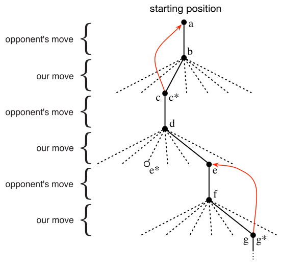
While we are playing, we change the values of the states in which we find ourselves during the game. We attempt to make them more accurate estimates of the probabilities of winning. To do this, we “back up” the value of the state after each greedy move to the state before the move, as suggested by the arrows in the figure. More precisely, the current value of the earlier state is updated to be closer to the value of the later state. This can be done by moving the earlier state’s value a fraction of the way toward the value of the later state. If we let $S_t$ denote the state before the greedy move, and $S_{t+1}$ the state after the move, then the update to the estimated value of $S_t$ , denoted $V(S_t)$, can be written as
$$ \begin{gather} V(S_t) \leftarrow V(S_t) + \alpha [ V(S_{t+1}) - V(S_t) ] \end{gather} $$where $\alpha$ is a small positive fraction called the step-size parameter, which influences the rate of learning. This update rule is an example of a temporal-difference learning method, so called because its changes are based on a difference, $V(S_{t+1}) - V(S_t)$, between estimates at two successive times.
The method described above performs quite well on this task. For example, if the step-size parameter is reduced properly over time, then this method converges, for any fixed opponent, to the true probabilities of winning from each state given optimal play by our player. Furthermore, the moves then taken (except on exploratory moves) are in fact the optimal moves against this (imperfect) opponent. In other words, the method converges to an optimal policy for playing the game against this opponent. If the step-size parameter is not reduced all the way to zero over time, then this player also plays well against opponents that slowly change their way of playing.
This example illustrates the differences between evolutionary methods and methods that learn value functions. To evaluate a policy an evolutionary method holds the policy fixed and plays many games against the opponent, or simulates many games using a model of the opponent. The frequency of wins gives an unbiased estimate of the probability of winning with that policy, and can be used to direct the next policy selection. But each policy change is made only after many games, and only the final outcome of each game is used: what happens during the games is ignored. For example, if the player wins, then all of its behavior in the game is given credit, independently of how specific moves might have been critical to the win. Credit is even given to moves that never occurred! Value function methods, in contrast, allow individual states to be evaluated. In the end, evolutionary and value function methods both search the space of policies, but learning a value function takes advantage of information available during the course of play. Recall that policy here is a rule that tells the player what move to make for every state of the game.
This simple example illustrates some of the key features of reinforcement learning methods. First, there is the emphasis on learning while interacting with an environment, in this case with an opponent player. Second, there is a clear goal, and correct behavior requires planning or foresight that takes into account delayed effects of one’s choices. For example, the simple reinforcement learning player would learn to set up multi-move traps for a shortsighted opponent. It is a striking feature of the reinforcement learning solution that it can achieve the effects of planning and lookahead without using a model of the opponent and without conducting an explicit search over possible sequences of future states and actions.
While this example illustrates some of the key features of reinforcement learning, it is so simple that it might give the impression that reinforcement learning is more limited than it really is. Although tic-tac-toe is a two-person game, reinforcement learning also applies in the case in which there is no external adversary, that is, in the case of a “game against nature.” Reinforcement learning also is not restricted to problems in which behavior breaks down into separate episodes, like the separate games of tic-tac-toe, with reward only at the end of each episode. It is just as applicable when behavior continues indefinitely and when rewards of various magnitudes can be received at any time. Reinforcement learning is also applicable to problems that do not even break down into discrete time steps like the plays of tic-tac-toe. The general principles apply to continuous-time problems as well, although the theory gets more complicated.
Tic-tac-toe has a relatively small, finite state set, whereas reinforcement learning can be used when the state set is very large, or even infinite. For example, Gerry Tesauro (1992, 1995) combined the algorithm described above with an artificial neural network to learn to play backgammon, which has approximately $10^{20}$ states. With this many states it is impossible ever to experience more than a small fraction of them. Tesauro’s program learned to play far better than any previous program and eventually better than the world’s best human players. The artificial neural network provides the program with the ability to generalize from its experience, so that in new states it selects moves based on information saved from similar states faced in the past, as determined by its network. How well a reinforcement learning system can work in problems with such large state sets is intimately tied to how appropriately it can generalize from past experience. It is in this role that we have the greatest need for supervised learning methods with reinforcement learning. Artificial neural networks and deep learning are not the only, or necessarily the best, way to do this.
In this tic-tac-toe example, learning started with no prior knowledge beyond the rules of the game, but reinforcement learning by no means entails a tabula rasa view of learning and intelligence. On the contrary, prior information can be incorporated into reinforcement learning in a variety of ways that can be critical for efficient learning. We also have access to the true state in the tic-tac-toe example, whereas reinforcement learning can also be applied when part of the state is hidden, or when different states appear to the learner to be the same.
Finally, the tic-tac-toe player was able to look ahead and know the states that would result from each of its possible moves. To do this, it had to have a model of the game that allowed it to foresee how its environment would change in response to moves that it might never make. Many problems are like this, but in others even a short-term model of the effects of actions is lacking. Reinforcement learning can be applied in either case. A model is not required, but models can easily be used if they are available or can be learned.
On the other hand, there are reinforcement learning methods that do not need any kind of environment model at all. Model-free systems cannot even think about how their environments will change in response to a single action. The tic-tac-toe player is model-free in this sense with respect to its opponent: it has no model of its opponent of any kind. Because models have to be reasonably accurate to be useful, model-free methods can have advantages over more complex methods when the real bottleneck in solving a problem is the difficulty of constructing a sufficiently accurate environment model. Model-free methods are also important building blocks for model-based methods. An exploration of model-free methods before more complex model-based methods is in order.
Reinforcement learning can be used at both high and low levels in a system. Although the tic-tac-toe player learned only about the basic moves of the game, nothing prevents reinforcement learning from working at higher levels where each of the “actions” may itself be the application of a possibly elaborate problem-solving method. In hierarchical learning systems, reinforcement learning can work simultaneously on several levels.
Working at higher levels might constitute, for example, initiating a plan consisting of more than one move towards a specific outcome.
Example
Consider an environment where our agent can observe the immediate result of an action – a color – and the rewards. (The world for the agent is partially observable.) The agent can perform three actions: wave, clap, and stand. The goal is to find the optimal policy – a way of selecting actions that gets you the most reward. Here is the structure of the environment, though the agent doesn’t have access to this:
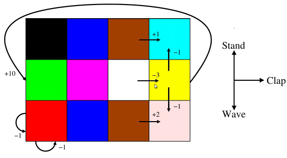
- the agent starts on green
- moves ‘off-the-board’ cause the agent to remain in the same place in the structure and receive a reward of $-1$
- the world here is deterministic rather than stochastic, e.g. clapping on green always results in purple
Formally, we have some knowns:
- observations - $\mathcal{O} = \{ \text{Blue}, \text{Red}, \dots\}$
- rewards in $\mathbb{R}$; note that the upper bound is not known a priori
- actions - $\mathcal{A} = \{Wave, Clap, Stand\}$ – note that the semantics available to the agent may be even more abstract and/or disconnected from the true semantics of the world, e.g. we may be limited to labels such as $\{action_A$, $action_B, \dots\}$.
And, so we have a sequence of the subsequence observation, action, and reward:
$$ \begin{gather} o_0, a_0, r_0, o_1, a_1, r_1, \dots \end{gather} $$We have discoverable unkowns:
- state space – $S = 4 \times 3$ grid
- reward function – $\mathcal{R}: \mathcal{S} \times \mathcal{A} \mapsto \mathbb{R}$
- observation function – $\mathcal{T} = \mathcal{S} \mapsto \mathcal{O}$ – state determines what color we observe
- probabilistic transition function – $\mathcal{P}: \mathcal{S} \times \mathcal{A} \mapsto \mathcal{S}$ – in this case, it is deterministic
Including the unknowns gives us the following account:
$$ \begin{gather} s_0, o_0, a_0, r_0, s_1, o_1, a_1, r_1, \dots \end{gather} $$- note that we now have states in the sequence
With all this information we can:
- obtain the observation with $o_i = \mathcal{T}(s_i)$
- get the reward with $r_i = \mathcal{R}(s_i, a_i)$
- use the transition function to determine the next state: $s_{i+1} = \mathcal{P}(s_i, a_i)$
We refer to these three equations as ’the model’.
Model-free algorithms don’t explicitly model $\mathcal{P}$, $\mathcal{R}$, and $\mathcal{T}$ as opposed to model-based algorithms which attempt to infer these.
See section 1.7 ‘Early History of Reinforcement Learning’ of Reinforcement Learning: An Introduction by Sutton & Barto for an excellent account of previous research.
Big Picture
Think of reinforcement learning as being one of several machine learning paradigms, with machine learning being a subfield of AI.
Taken all together these types of learning include:
- supervised learning – learning from labeled examples
- unsupervised learning – cluster from unlabeled examples
- reinforcement learning – learn from interaction
The problem itself will determine the type of learning involved…
Reinforcement learning problems are characterized by the following:
- closed-loop – you take an action and that affects the next observation that you get
- select own actions
- sequential (time-delayed)
Given a reinforcement learning problem, there are many different approaches, e.g. evolutionary approaches.
For pedagogical reasons consider the following simplified formalism. Consider again the previous example:
- state - $\mathcal{S} = \{ \text{Blue}, \text{Red}, \dots\}$
- rewards in $\mathbb{R}$
- actions - $\mathcal{A} = \{Wave, Clap, Stand\}$
Note that we now have states that are uniquely identifiable by the associated observation.
This results in a simplification of the unknowns. We now have the following:
- reward function – $\mathcal{R}: \mathcal{S} \times \mathcal{A} \mapsto \mathbb{R}$
- probabilistic transition function – $\mathcal{P}: \mathcal{S} \times \mathcal{A} \mapsto \mathcal{S}$ – remember, it is deterministic
Note that there is no observation function.
Now our model is simply the reward function and the state transition function:
- get the reward with $r_i = \mathcal{R}(s_i, a_i)$
- use the transition function to determine the next state: $s_{i+1} = \mathcal{P}(s_i, a_i)$
From the agent’s perspective only the policy is under the control of the agent; all the functions discussed previously are given and fixed. The only decision that the agent has to make is what function it should use to select actions for each state. The state function and reward functions pre-exist. The value function expresses how good it is to be in a particular state in the long run.
On-policy learning algorithms are important – learning how to act and how good it is to act according to the policy you’re currently using. There are also off-policy learning algorithms.
If you have a really good reinforcement learning agent, you can program it to behave well by just specifying goals to it. For example, you might need your house cleaned; so, you make this request of the agent without having to specify exactly how to do this, e.g. ’take the mop in hand, go to the dining room, etc.’
In practice, you need to pick a representation and a reward function.
The art is in picking the representation and picking the reward function and the science is analysis.
Tabular Methods
Tabular methods are used when we have a finite state and action space, typically small, that can be represented by a table. In this case, the methods can often find exact solutions, that is, they can often find exactly the optimal value function and the optimal policy. This contrasts with the approximate methods, which only find approximate solutions, but which in return can be applied effectively to much larger problems.
Two Special Cases
Consider two important special cases of the reinforcement learning problem:
- problems in which there is only a single state, called bandit problems.
- the general problem formulation—finite Markov decision processes—and its main ideas including Bellman equations and value functions.
The latter of which includes three fundamental classes of methods: dynamic programming, Monte Carlo methods, and temporal- difference learning. Each class of methods has its strengths and weaknesses. Dynamic programming methods are well developed mathematically, but require a complete and accurate model of the environment. Monte Carlo methods don’t require a model and are conceptually simple, but are not well suited for step-by-step incremental computation. Finally, temporal-difference methods require no model and are fully incremental, but are more complex to analyze. The methods also differ in several ways with respect to their efficiency and speed of convergence.
These three classes of methods can be combined to obtain the best features of each of them. In fact temporal-difference learning methods can be combined with model learning and planning methods (such as dynamic programming) for a complete and unified solution to the tabular reinforcement learning problem.